1
Mobile Robot Localisation
1.1 Introduction
Navigation is one of, if not, the most challenging problem faced by an
AMR
and for the robot to be
able to successfully navigate its environment, it requires four
- Perception
-
the robot must be able to interpret its sensors to extract meaningful data,
- Localisation
-
the robot must be able to determine its position within the environment,
- Cognition
-
the robot must be able to decide how to act to achieve its goals,
- Motion control
-
the robot must be able to modulate its motor outputs to achieve the desired trajectory.
Of these four
The structure of the chapter is as follows:
-
We will describe how sensor and effector uncertainty is responsible for the difficulties of localisation in Section 1.2 ,
-
Then, in Section 1.3 , we will have a look at the two
(2) extreme approaches to dealing with the challenge of robot localisation [6]:-
Avoiding localisation altogether,
-
Performing explicit map-based localisation
-
-
The remainder of the chapter discusses the question of representation, which we will have a look at different case studies of successful localisation systems using a variety of representations and techniques to achieve AMR localisation.
1.2 The problems of Noise and Aliasing
If one could attach an accurate
Global Positioning System (GPS)
sensor to an
AMR
, much of the
localisation problem would be obviated.
GPS
would then inform the robot of its
would
Unfortunately,
such
a
sensor
is
NOT
currently
practical.
In addition, GPS cannot function indoors or in obstructed areas and are therefore limited in their workspace. But, looking beyond the limitations of GPS , localisation implies more than knowing one’s absolute position in the Earth’s reference frame.
Consider a robot which is interacting with humans. This robot may need to identify its absolute position, but its relative position with respect to target humans is also equally important. Its localisation task can include:
-
identifying humans using its sensor array [9],
-
then computing its relative position to the humans.
Furthermore,
during
operation
a
robot
will
select
a
strategy
for
achieving
its
goals.
If
it
intends
to
reach
a
particular
location,
then
localisation
may
not
be
enough.
The
robot
may
need
to
acquire
or
build
an
environmental
model,
Localisation means more than simply determining an absolute pose in space. It means building a map, then identifying the robot’s position relative to that map.
Clearly, the robot’s sensors and effectors play an integral role in all the above forms of localisation. It is because of the inaccuracy and incompleteness of these sensors and effectors localisation poses difficult challenges.
1.2.1 Sensor Noise
Sensors are the fundamental robot input for the process of perception, and therefore the degree to which sensors can
discriminate world state is critical. Sensor noise produces a
Often, the source of sensor noise problems is that some environmental features are not captured by the robot’s representation and are thus overlooked.
For
example,
a
vision
system
used
for
indoor
navigation

Illumination dependency is only one example of the apparent noise in a vision-based sensor system [10]. Picture jitter, signal gain, blooming and blurring are all additional sources of noise, potentially reducing the useful content of a colour video image.
Consider the noise level of ultrasonic range-measuring sensors, such as sonars, as we discussed previously. When a sonar transducer
emits sound towards a relatively smooth and angled surface, much of the signal will coherently reflect away, failing to generate a
return echo. Depending on the material characteristics, a small amount of energy may return nonetheless. When this level is close
to the gain threshold of the sonar sensor, then the sonar will, at times, succeed and, at other times, fail to detect the object.
From the robot’s perspective, a virtually unchanged environmental state will result in two
one short, and one long which causes an nondeterministic behaviour.
The
poor
Signal-to-Noise
Ratio
(SNR)
of
a
sonar
sensor
is
further
confounded
by
interference
between
multiple
sonar
emitters.
Often,
research
robots
have
between
12
to
48
sonars
on
a
single
platform.
In
acoustically
reflective
environments,
multipath
interference
In
conclusion,
sensor
noise
reduces
the
useful
information
content
of
sensor
readings.
Clearly,
the
solution
is
to
take
multiple
readings
into
account,
employing
temporal
fusion
or
multi-sensor
fusion
1.2.2 Sensor Aliasing
Aliasing
is
the
second
major
shortcoming
of
AMR
sensors
which
cause
them
to
give
little
information
content,
further
amplifying
the
problem
of
Information : The Human Experience
The problem, known as sensor aliasing, is a phenomenon that humans seldom encounter. The human sensory system, particularly the visual system, tends to receive unique inputs in each unique local state within normal usage [12]. In other words, every different place looks different. The power of this unique mapping is only apparent when one considers situations where this fails to hold.
Consider moving through an unfamiliar building that is completely dark. When the visual system sees only black, one’s localisation system quickly degrades. Another useful example is that of a human-sized maze made from tall hedges. Such mazes have been created for centuries, and humans find them extremely difficult to solve without landmarks or clues because, without visual uniqueness, human localisation competence degrades rapidly.
In
robots,
the
non-uniqueness
of
sensors
readings,
or
sensor
aliasing,
A classical problem with sonar-based robots involves distinguishing between humans and inanimate objects in an indoor setting [ 14 , 15 ].
When facing an apparent obstacle in front of itself, should the robot say “Excuse me” because the obstacle may be a moving human, or should the robot plan a path around the object because it may be a cardboard box?
With sonar alone, these states are aliased and differentiation is impossible.
The
navigation
problem
due
to
sensor
aliasing
is
that,
even
with
noise-free
sensors,
the
amount
of
information
is
generally
1.2.3 Effector Noise
The challenges of localisation does NOT lie with sensor technologies alone. Just as robot sensors are noisy, limiting the information content of the signal, so do the robot effectors.
A single action taken by a AMR may have several different possible results, even though from the robot’s point of view the initial state before the action was taken is well-known.
In
short,
AMR
effectors
introduce
uncertainty
about
future
state.

First,
however,
it
is
important
to
understand
the
precise
nature
of
the
effector
noise
that
impacts
AMR
.
It
is
important
to
note
that,
from
the
robot’s
point
of
view,
this
error
in
motion
is
viewed
as
For instance, the robot does NOT model the fact that the floor may be sloped, the wheels may slip, and a human may push the robot.
All of these unmodeled sources of error result in:
-
inaccuracy between the physical motion of the robot,
-
the intended motion of the robot, and the
-
proprioceptive sensor estimates of motion.
In
odometry
and
dead
reckoning
In the following we will concentrate on odometry based on the wheel sensor readings of a differential drive robot only [16].
There are many sources of odometric error, from environmental factors to resolution:
-
Limited resolution during integration
11 11 time increments, measurement resolution -
Misalignment of wheels causing
deterministic error, -
Unequal wheel diameter, which again, causing
deterministic error, -
Unequal floor contact, which can cause
slipping during operation.
Some
of
the
errors
might
be
deterministic
- Range error
-
Integrated path length of the robot movement, as in the sum of wheel motion.
- Turn error
-
Similar to range error, but for turns which are difference of the wheel motions.
- Drift error
-
difference in the error of the wheels leads to an error in the robot’s angular orientation.
Over long periods of time, turn and drift errors far outweigh range errors, as their contribute to the overall position error is non-linear. Consider a robot, whose position is initially perfectly well-known, moving forward in a straight line along the x axis. The error in the y -position introduced by a move of meters will have a component of , which can be quite large as the angular error grows. Over time, as an AMR moves about the environment, the rotational error between its internal reference frame and its original reference frame grows quickly. As the robot moves away from the origin of these reference frames, the resulting linear error in position grows quite large. It is instructive to establish an error model for odometric accuracy and see how the errors propagate over time.
1.2.4 An Error Model for Odometric Position Estimation
Generally the pose (position) of a robot is represented by the vector
For a differential drive robot the position can be estimated starting from a known position by integrating the movement (summing the incremental travel distances). For a discrete system with a fixed sampling interval the incremental travel distances are:
As we discussed earlier, odometric position updates can give only a very rough estimate of the actual position. Due to integration errors of the uncertainties of p and the motion errors during the incremental motion (s ;s ) the position error based on odometry integration rl grows with time. In the next step we will establish an error model for the integrated position p’ to obtain the of the odometric position estimate. To do so, we assume that at the covariance matrix starting point the initial covariance matrix is known. For the motion increment p (s ;s ) we assume the following covariance matrix : rl where s and s are the distances travelled by each wheel, and k , k are error constants rlrl representing the non-deterministic parameters of the motor drive and the wheel-floor inter- action. As you can see in equation (5.8) we made the following assumption
-
The two
(2) errors of the individually driven wheels are independent.13 13 If there is more knowledge regarding the actual robot kinematics, the correlation terms of the covariance matrix could also be used. -
The errors are proportional to the
absolute value of the travelled distances .
These assumptions, while NOT perfect in the slightest, are nevertheless suitable and will therefore be used for the further development of the error model.
The
The values for the error constants and depend on the robot and the environment and should be experimentally determined by performing and analysing representative movements.
If
we
assume
that
and
are
The covariance matrix is, of course, always given by the p p’
1.3 Localisation v. Hard-Coded Navigation
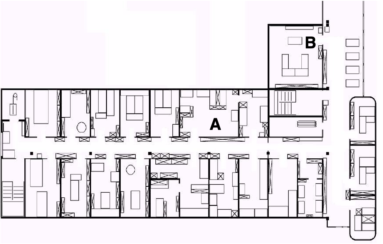
Fig.
1.3
depicts
a
standard
indoor
environment
an
AMR
is
set
to
navigate.
Now,
suppose
an
AMR
in
question
must
deliver
messages
between
two
These
are
rooms
In creating a navigation system for this task, it is clear the AMR will need sensors and a motion control system. Sensors are required to avoid hitting moving obstacles such as humans, and some motion control system is required so that the robot can actively move.
It
is
less
evident,
however,
whether
or
not
this
AMR
will
require
a
localisation
system.
Localisation
may
seem
mandatory
to
successfully
navigate
between
the
two
An
alternative,
adopted
by
the
behaviour-based
community,
suggests
that,
since
sensors
and
effectors
are
noisy
and
information-limited,
one
should
In its essence, this approach avoids explicit reasoning about localisation and position, and therefore generally avoids explicit path planning as well.
This
technique
is
based
on
a
idea
that,
there
exists
a
procedural
solution
to
the
particular
navigation
problem
at
hand.
For
example,
in
Fig.
1.3
,
the
behavioralist
approach
to
navigating
from
Room
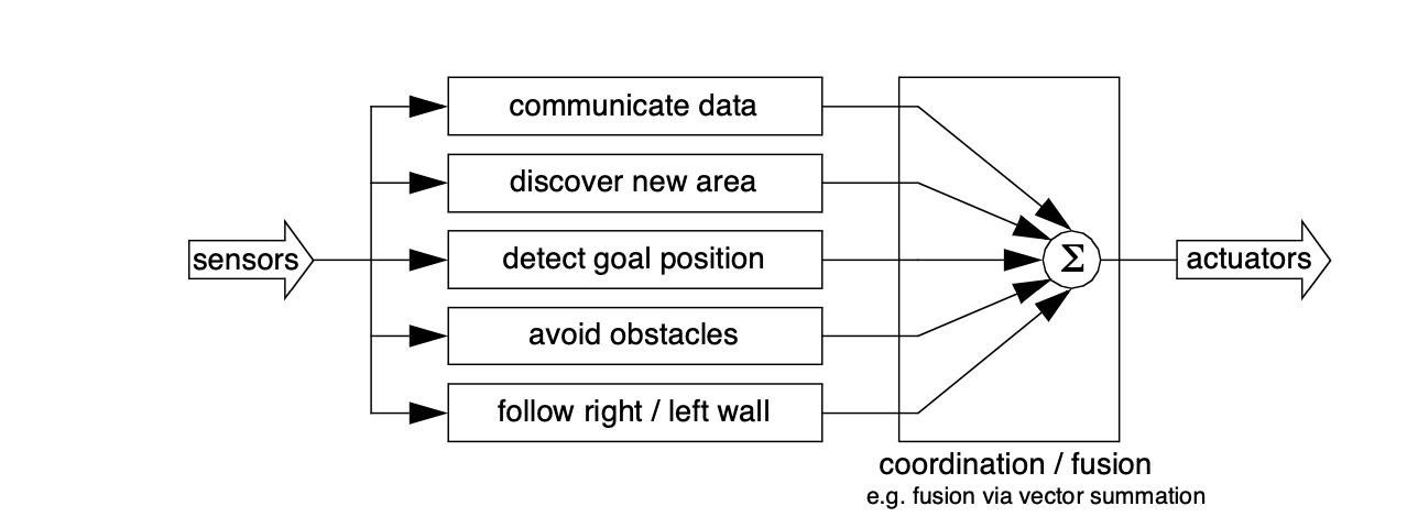
The architecture of this solution to a specific navigation problem is shown in Fig. 1.4 . The key advantage of this method is that, when possible, it may be implemented very quickly for a single environment with a small number of goal positions. It suffers from some disadvantages, however.
-
The method does not directly scale to other environments or to larger environments. Often, the navigation code is location-specific, and the same degree of coding and debugging is required to move the robot to a new environment.
-
The underlying procedures, such as left-wall-follow, must be carefully designed to produce the desired behaviour. This task may be time-consuming and is heavily dependent on the specific robot hardware and environmental characteristics.
-
A behaviour-based system may have multiple active behaviors at any one time. Even when individual behaviours are tuned to optimise performance, this fusion and rapid switching between multiple behaviors can negate that fine-tuning. Often, the addition of each new incremental behavior forces the robot designer to re-tune all of the existing behaviors again to ensure that the new interactions with the freshly introduced behavior are all stable
In contrast to the behaviour-based approach, the map-based approach includes both localisation and cognition modules shown in Fig. 1.5 .
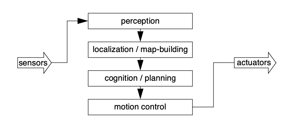
In
map-based
navigation,
the
robot
-
The explicit, map-based concept of position makes the system’s belief about position transparently available to the human operators.
-
The existence of the map itself represents a medium for communication between human and robot as the human can simply give the robot a new map if the robot goes to a new environment.
-
The map, if created by the robot, can be used by humans as well, achieving two uses.
The map-based approach will require more up-front development effort to create a navigating AMR . The hope is that the development effort results in an architecture which can successfully map and navigate a variety of environments, thereby compensating for the up-front design cost over time.
Of
course
the
primary
risk
of
the
map-based
approach
is
that
an
internal
representation,
rather
than
the
real
world
itself,
is
being
constructed
and
trusted
by
the
robot.
If
that
model
diverges
from
reality,
In the remainder of this chapter, we focus on a discussion of map-based approaches and, specifically, the localisation component of these techniques. These approaches are particularly appropriate for study given their significant recent successes in enabling AMR to navigate a variety of environments, from academic research buildings to factory floors and museums around the world.
1.4 Representing Belief
The
fundamental
issue
which
differentiates
different
types
of
map-based
localisation
systems
is
the
issue
of
- 1.
- Representation of the environment,
- 2.
- The map.
What aspects of the environment are contained in this map? At what level of fidelity does the map represent the environment? These are the design questions for map representation.
The
robot
must
also
have
a
representation
of
its
Does the robot identify a single unique position as its current position, or does it describe its position in terms of a set of possible positions? If multiple possible positions are expressed in a single belief, how are those multiple positions ranked, if at all?
These
are
the
design
questions
for
belief
representation.
Decisions
along
these
two
We will start by discussing belief representation. The first major branch in the classification of belief representation systems differentiates between single hypothesis and multiple hypothesis belief systems.
- Single
-
Former covers solutions in which the robot postulates its unique position,
- Multiple
-
Enables a AMR to describe the degree to which it is uncertain about its position.
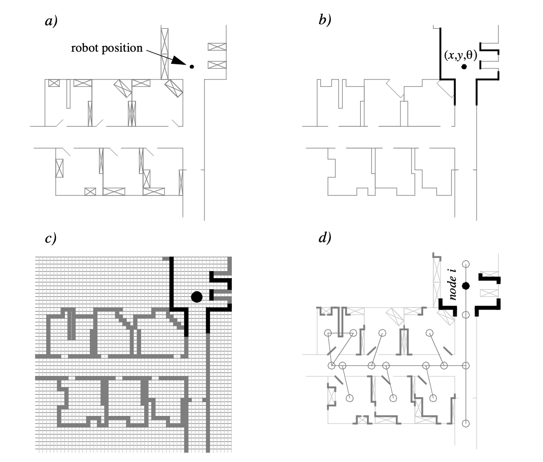
A sampling of different belief and map representations is shown in figure 5.9.
1.4.1 Single Hypothesis Belief
The single hypothesis belief representation is the most direct possible postulation of an AMR ’s position [18].
Given some environmental map, the robot’s belief about position is expressed as a single unique point on the map.
In
Fig.
1.7
,
three
The
principal
advantage
of
the
single
hypothesis
representation
of
position
stems
from
the
fact
that,
given
a
unique
belief,
there
is
Just as decision-making is facilitated by a single-position hypothesis, so updating the robot’s belief regarding position is also facilitated, since the single position must be updated by definition to a new, single position. The challenge with this position update approach, which ultimately is the principal disadvantage of single-hypothesis representation, is that robot motion often induces uncertainty due to effectory and sensory noise.
Forcing the position update process to always generate a single hypothesis of position is challenging and, often, impossible.
1.4.2 Multiple Hypothesis Belief
In
the
case
of
multiple
hypothesis
beliefs
regarding
position,
the
robot
tracks
NOT
just
a
single
possible
position
but
a
possibly
This multiple hypothesis representation communicates the set of possible robot positions geometrically, with no preference ordering over the positions. Each point in the map is simply either contained by the polygon and, therefore, in the robot’s belief set, or outside the polygon and thereby excluded. Mathematically, the position polygon serves to partition the space of possible robot positions. Such a polygonal representation of the multiple hypothesis belief can apply to a continuous, geometric map of the environment or, alternatively, to a tessellated, discrete approximation to the continuous environment.
It may be useful, however, to incorporate some ordering on the possible robot positions, capturing the fact that some robot positions are likelier than others. A strategy for representing a continuous multiple hypothesis belief state along with a preference ordering over possible positions is to model the belief as a mathematical distribution. For example, [42,47] notate the robot’s position belief using an X,Y point in the two-dimensional environment as the mean plus a standard deviation parameter , thereby defining a Gaussian distribution. The intended interpretation is that the distribution at each position represents the probability assigned to the robot being at that location. This representation is particularly amenable to mathematically defined tracking functions, such as the Kalman Filter, that are designed to operate efficiently on Gaussian distributions.
An alternative is to represent the set of possible robot positions, not using a single Gaussian probability density function, but using discrete markers for each possible position. In this case, each possible robot position is individually noted along with a confidence or probability parameter (See Fig. (5.11)). In the case of a highly tessellated map this can result in thousands or even tens of thousands of possible robot positions in a single belief state.
The key advantage of the multiple hypothesis representation is that the robot can explicitly maintain uncertainty regarding its position. If the robot only acquires partial information regarding position from its sensors and effectors, that information can conceptually be incorporated in an updated belief.
A more subtle advantage of this approach revolves around the robot’s ability to explicitly measure its own degree of uncertainty regarding position. This advantage is the key to a class of localisation and navigation solutions in which the robot not only reasons about reaching a particular goal, but reasons about the future trajectory of its own belief state. For instance, a robot may choose paths that minimise its future position uncertainty. An example of this approach is [90], in which the robot plans a path from point A to B that takes it near a series of landmarks in order to mitigate localisation difficulties. This type of explicit reasoning about the effect that trajectories will have on the quality of localisation requires a multiple hypothesis representation.
One of the fundamental disadvantages of the multiple hypothesis approaches involves decision-making. If the robot represents its position as a region or set of possible positions, then how shall it decide what to do next? Figure 5.11 provides an example. At position 3, the robot’s belief state is distributed among 5 hallways separately. If the goal of the robot is to travel down one particular hallway, then given this belief state what action should the robot choose?
The challenge occurs because some of the robot’s possible positions imply a motion trajectory that is inconsistent with some of its other possible positions. One approach that we will see in the case studies below is to assume, for decision-making purposes, that the robot is physically at the most probable location in its belief state, then to choose a path based on that current position. But this approach demands that each possible position have an associated probability.
In general, the right approach to such a decision-making problems would be to decide on trajectories that eliminate the ambiguity explicitly. But this leads us to the second major disadvantage of the multiple hypothesis approaches. In the most general case, they can be computationally very expensive. When one reasons in a three dimensional space of discrete possible positions, the number of possible belief states in the single hypothesis case is limited to the number of possible positions in the 3D world. Consider this number to be N. When one moves to an arbitrary multiple hypothesis representation, then the number of posN sible belief states is the power set of N, which is far larger: 2 . Thus explicit reasoning about the possible trajectory of the belief state over time quickly becomes computationally untenable as the size of the environment grows. There are, however, specific forms of multiple hypothesis representations that are somewhat more constrained, thereby avoiding the computational explosion while allowing a limited type of multiple hypothesis belief. For example, if one assumes a Gaussian distribution of probability centered at a single position, then the problem of representation and tracking of belief becomes equivalent to Kalman Filtering, a straightforward mathematical process described below. Alternatively, a highly tessellated map representation combined with a limit of 10 possible positions in the belief state, results in a discrete update cycle that is, at worst, only 10x more computationally expensive than single hypothesis belief update.
In conclusion, the most critical benefit of the multiple hypothesis belief state is the ability to maintain a sense of position while explicitly annotating the robot’s uncertainty about its own position. This powerful representation has enabled robots with limited sensory information to navigate robustly in an array of environments, as we shall see in the case studies below.
1.5 Representing Maps
The problem of representing the environment in which an AMR moves is a dual of the problem of representing the robot’s possible position or positions. Decisions made regarding the environmental representation can have impact on the choices available for robot position representation.
Often the fidelity of the position representation is bounded by the fidelity of the map.
There
are
three
- 1.
- The precision of the map must appropriately match the precision with which the robot needs to achieve its goals.
- 2.
- The precision of the map and the type of features represented must match the precision and data types returned by the robot’s sensors.
- 3.
- The complexity of the map representation has direct impact on the computational complexity of reasoning about mapping, localisation and navigation.
Using the aforementioned criteria, we identify and discuss critical design choices in creating a map representation. Each such choice has great impact on the relationships, and on the resulting robot localisation architecture. As we will see, the choice of possible map representations is broad, if not expansive. Selecting an appropriate representation requires understanding all of the trade-offs inherent in that choice as well as understanding the specific context in which a particular AMR implementation must perform localisation.
1.5.1 Continuous Representation
A
continuous-valued
map
is
one
method
for exact
decomposition
of
the
environment.
The
position
of
environmental
features
can
be
mapped
precisely
in
continuous
space.
AMR
implementations
to
date
use
continuous
maps
only
in
two
A common approach is to combine the exactness of a continuous representation with the compactness of the closed world assumption. This means that one assumes the representation will specify all environmental objects in the map, and that any area in the map which is devoid of objects has no objects in the corresponding portion of the environment. Therefore, the total storage needed in the map is proportional to the density of objects in the environment, and a sparse environment can be represented by a low-memory map.
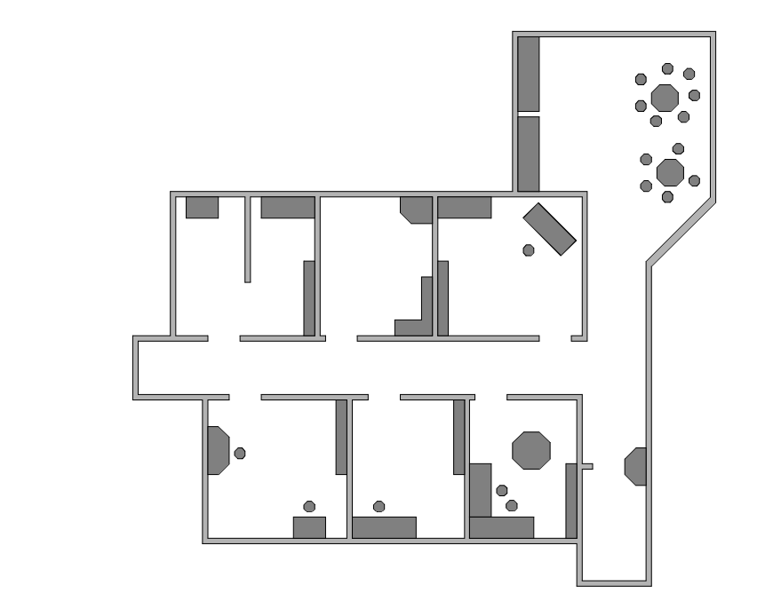
One example of such a representation, shown in Fig. 1.9 , is a 2D representation in which polygons represent all obstacles in a continuos-valued coordinate space. This is similar to the method used by Latombe [5, 113] and others to represent environments for AMR path planning techniques. In the case of [5, 113], most of the experiments are in fact simulations run exclusively within the computer’s memory. Therefore, no real effort would have been expended to attempt to use sets of polygons to describe a real-world environment, such as a park or office building.
In
other
work
in
which
real
environments
must
be
captured
by
the
maps,
there
seems
to
be
a
trend
towards
It should be immediately apparent that geometric maps can capably represent the physical locations of objects without referring to their texture, colour, elasticity, or any other such secondary features that do not related directly to position and space.
In
addition
to
this
level
of
abstraction,
an
AMR
map
can
further
reduce
memory
usage
by
capturing
only
One
excellent
example
involves
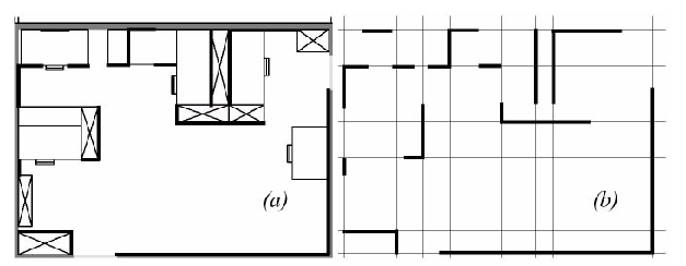
Fig. 1.10 shows a map of an indoor environment at EPFL using a continuous line representation. Note that the only environmental features captured by the map are straight lines, such as those found at corners and along walls. This represents not only a sampling of the real world of richer features, but also a simplification, for an actual wall may have texture and relief that is not captured by the mapped line. The impact of continuos map representations on position representation is primarily positive. In the case of single hypothesis position representation, that position may be specified as any continuous-valued point in the coordinate space, and therefore extremely high accuracy is possible. In the case of multiple hypothesis position representation, the continuous map enables two types of multiple position representation. In one case, the possible robot position may be depicted as a geometric shape in the hyperplane, such that the robot is known to be within the bounds of that shape. This is shown in Figure 5.30, in which the position of the robot is depicted by an oval bounding area. Yet, the continuous representation does not disallow representation of position in the form of a discrete set of possible positions. For instance, in [111] the robot position belief state is captured by sampling nine continuous-valued positions from within a region near the robot’s best known position. This algorithm captures, within a continuous space, a discrete sampling of possible robot positions. In summary, the key advantage of a continuous map representation is the potential for high accuracy and expressiveness with respect to the environmental configuration as well as the robot position within that environment. The danger of a continuous representation is that the map may be computationally costly. But this danger can be tempered by employing abstraction and capturing only the most relevant environmental features. Together with the use of the closed world assumption, these techniques can enable a continuous-valued map to be no more costly, and sometimes even less costly, than a standard discrete representation.
1.5.2 Decomposition Methods
In previous section, we discussed one method of simplification, in which the continuous map representation contains a set of infinite lines which approximate real-world environmental lines based on a two-dimensional slice of the world.
Basically this transformation from the real world to the map representation is a filter that removes all non-straight data and furthermore extends line segment data into infinite lines that require fewer parameters.
A more dramatic form of simplification is abstraction:
a general decomposition and selection of environmental features.
In this section, we explore decomposition as applied in its more extreme forms to the question of map representation. Why would one radically decompose the real environment during the design of a map representation? The immediate disadvantage of decomposition and abstraction is the loss of fidelity between the map and the real world. Both qualitatively, in terms of overall structure, and quantitatively, in terms of geometric precision, a highly abstract map does not compare favourably to a high-fidelity map.
Despite this disadvantage, decomposition and abstraction may be useful if the abstraction can be planned carefully so as to capture the relevant, useful features of the world while discarding all other features. The advantage of this approach is that the map representation can potentially be minimised. Furthermore, if the decomposition is hierarchical, such as in a pyramid of recursive abstraction, then reasoning and planning with respect to the map rep- resentation may be computationally far superior to planning in a fully detailed world model.
A standard, lossless form of opportunistic decomposition is termed exact cell decomposition. This method, introduced by [5], achieves decomposition by selecting boundaries between discrete cells based on geometric criticality.
Figure 5.14 depicts an exact decomposition of a planar workspace populated by polygonal obstacles. The map representation tessellates the space into areas of free space. The representation can be extremely compact because each such area is actually stored as a single node, shown in the graph at the bottom of Figure 5.14.
The underlying assumption behind this decomposition is that the particular position of a robot within each area of free space does not matter. What matters is the robot’s ability to traverse from each area of free space to the adjacent areas. Therefore, as with other representations we will see, the resulting graph captures the adjacency of map locales. If indeed the assumptions are valid and the robot does not care about its precise position within a single area, then this can be an effective representation that nonetheless captures the connectivity of the environment.
Such an exact decomposition is not always appropriate. Exact decomposition is a function of the particular environment obstacles and free space. If this information is expensive to collect or even unknown, then such an approach is not feasible.
An alternative is fixed decomposition, in which the world is tessellated, transforming the continuos real environment into a discrete approximation for the map. Such a transforma- tion is demonstrated in Figure 5.15, which depicts what happens to obstacle-filled and free areas during this transformation. The key disadvantage of this approach stems from its in- exact nature. It is possible for narrow passageways to be lost during such a transformation, as shown in Figure 5.15. Formally this means that fixed decomposition is sound but not complete. Yet another approach is adaptive cell decomposition as presented in Figure 5.16.
The concept of fixed decomposition is extremely popular in AMR ics; it is perhaps the single most common map representation technique currently utilised. One very popular
version of fixed decomposition is known as the occupancy grid representation [91]. In an occupancy grid, the environment is represented by a discrete grid, where each cell is either filled (part of an obstacle) or empty (part of free space). This method is of particular value when a robot is equipped with range-based sensors because the range values of each sensor, combined with the absolute position of the robot, can be used directly to update the filled/ empty value of each cell. In the occupancy grid, each cell may have a counter, whereby the value 0 indicates that the cell has not been "hit" by any ranging measurements and, therefore, it is likely free space. As the number of ranging strikes increases, the cell’s value is incremented and, above a cer- tain threshold, the cell is deemed to be an obstacle. By discounting the values of cells over time, both hysteresis and the possibility of transient obstacles can be represented using this occupancy grid approach. Figure 5.17 depicts an occupancy grid representation in which the darkness of each cell is proportional to the value of its counter. One commercial robot that uses a standard occupancy grid for mapping and navigation is the Cye robot [112].
There remain two main disadvantages of the occupancy grid approach. First, the size of the map in robot memory grows with the size of the environment and, if a small cell size is used, this size can quickly become untenable. This occupancy grid approach is not compatible with the closed world assumption, which enabled continuous representations to have poten- tially very small memory requirements in large, sparse environments. In contrast, the occu- pancy grid must have memory set aside for every cell in the matrix. Furthermore, any fixed decomposition method such as this imposes a geometric grid on the world a priori, regard- less of the environmental details. This can be inappropriate in cases where geometry is not the most salient feature of the environment. For these reasons, an alternative, called topological decomposition, has been the subject of some exploration in AMR ics. Topological approaches avoid direct measurement of geometric environmental qualities, instead concentrating on characteristics of the environ- ment that are most relevant to the robot for localisation. Formally, a topological representation is a graph that specifies two things: nodes and the connectivity between those nodes. Insofar as a topological representation is intended for the use of a AMR , nodes are used to denote areas in the world and arcs are used to denote adjacency of pairs of nodes. When an arc connects two nodes, then the robot can traverse from one node to the other without requiring traversal of any other intermediary node. Adjacency is clearly at the heart of the topological approach, just as adjacency in a cell de- composition representation maps to geometric adjacency in the real world. However, the topological approach diverges in that the nodes are not of fixed size nor even specifications of free space. Instead, nodes document an area based on any sensor discriminant such that the robot can recognise entry and exit of the node. Figure 5.18 depicts a topological representation of a set of hallways and offices in an indoor
environment. In this case, the robot is assumed to have an intersection detector, perhaps us- ing sonar and vision to find intersections between halls and between halls and rooms. Note that nodes capture geometric space and arcs in this representation simply represent connec- tivity. Another example of topological representation is the work of Dudek [49], in which the goal is to create a AMR that can capture the most interesting aspects of an area for human consumption. The nodes in Dudek’s representation are visually striking locales rather than route intersections. In order to navigate using a topological map robustly, a robot must satisfy two constraints. First, it must have a means for detecting its current position in terms of the nodes of the to- pological graph. Second, it must have a means for traveling between nodes using robot mo- tion. The node sizes and particular dimensions must be optimised to match the sensory discrimination of the AMR hardware. This ability to "tune" the representation to the robot’s particular sensors can be an important advantage of the topological approach. How- ever, as the map representation drifts further away from true geometry, the expressiveness of the representation for accurately and precisely describing a robot position is lost. Therein lies the compromise between the discrete cell-based map representations and the topological representations. Interestingly, the continuous map representation has the potential to be both compact like a topological representation and precise as with all direct geometric rep- resentations. Yet, a chief motivation of the topological approach is that the environment may contain im- portant non-geometric features - features that have no ranging relevance but are useful for localisation. In Chapter 4 we described such whole-image vision-based features. In contrast to these whole-image feature extractors, often spatially localised landmarks are artificially placed in an environment to impose a particular visual-topological connectivity upon the environment. In effect, the artificial landmark can impose artificial structure. Ex- amples of working systems operating with this landmark-based strategy have also demon- strated success. Latombe’s landmark-based navigation research 89 has been implemented on real-world indoor AMR s that employ paper landmarks attached to the ceiling as the locally observable features. Chips the museum robot is another robot that uses man- made landmarks to obviate the localisation problem. In this case, a bright pink square serves as a landmark with dimensions and color signature that would be hard to accidentally repro- duce in a museum environment [88]. One such museum landmark is shown in Figure (5.19). In summary, range is clearly not the only measurable and useful environmental value for a AMR . This is particularly true due to the advent of color vision as well as laser rangefinding, which provides reflectance information in addition to range information. Choosing a map representation for a particular AMR requires first understanding the sensors available on the AMR and second understanding the AMR ’s function- al requirements (e.g. required goal precision and accuracy).
1.5.3 Current Challenges
Previous section describe major design decisions with regards to map representation choices. There are, however, fundamental real-world features which AMR map representations do not work as well. These continue to be the subject of open research, and several such challenges are described below.
The real world is
-
moving people,
-
cars,
-
strollers, and
-
transient obstacles.
This is particularly true when one considers a home setting with which domestic robots will someday need to contend.
The map representations described previously do not, in general, have
Usually, the assumption behind the above map representations is that all objects on the map are effectively
As
vision
sensing
provides
more
robust
and
more
informative
content
regarding
the
transience
and
motion
details
of
objects
in
the
world,
researchers
will
in
time
propose
representations
that
make
use
of
that
information.
A
classic
example
involves
occlusion
by
human
crowds.
Museum
tour
guide
robots
A second open challenge in AMR localisation involves the traversal of open spaces. Existing localisation techniques generally depend on local measures such as range, thereby demanding environments that are somewhat densely filled with objects that the sensors can detect and measure. Wide open spaces such as parking lots, fields of grass and indoor open-spaces such as those found in convention centres or expos pose a difficulty for such systems due to their relative sparseness. Indeed, when populated with humans, the challenge is exacerbated because any mapped objects are almost certain to be occluded from view by the people.
Once again, more recent technologies provide some hope for overcoming these limitations. Both vision and state-of-the-art laser range-finding devices offer outdoor performance with ranges of up to a hundred meters and more. Of course, GPS performs even better. Such long-range sensing may be required for robots to localise using distant features.
This trend teases out a hidden assumption underlying most topological map representations. Usually, topological representations make assumptions regarding spatial locality:
a node contains objects and features that are themselves within that node.
The process of map creation therefore involves making nodes which are, in their own self-contained way, recognizable by virtue of
the objects contained within the node. Therefore, in an indoor environment, each room can be a separate node. This is a
reasonable assumption as each room will have a layout and a set of belongings that are
However, consider the outdoor world of a wide-open park.
Where should a single node end and the next node begin?
The answer is unclear as objects which are far away from the current node, or position, can give information for the localisation process. For example, the hump of a hill at the horizon, the position of a river in the valley and the trajectory of the Sun all are non-local features that have great bearing on one’s ability to infer current position.
The spatial locality assumption is violated and, instead, replaced by a visibility criterion:
the node or cell may need a mechanism for representing objects that are measurable and visible from that cell.
Once
again,
as
sensors
and
outdoor
locomotion
mechanisms
improve,
there
will
be
greater
urgency
to
solve
problems
associated
with
localisation
in
wide-open
settings,
with
and
without
GPS-type
global
localisation
sensors.
We end this section with one final open challenge that represents one of the fundamental ac- ademic research questions of robotics: sensor fusion .
Information : Sensor Fusion
A variety of measurement types are possible using off-the-shelf robot sensors, including heat, range, acoustic and light-based reflectivity, color, texture, friction, etc. Sensor fusion is a research topic closely related to map representation. Just as a map must embody an environment in sufficient detail for a robot to perform localisation and reasoning, sensor fusion demands a representation of the world that is sufficiently general and expressive that a variety of sensor types can have their data correlated appropriately, strengthening the resulting percepts well beyond that of any individual sensor’s readings.
An implementation example implementation of sensor fusion to date is that of neural network classifier. Using this technique, any number and any type of sensor values may be jointly combined in a network that will use whatever means necessary to optimise its classification accuracy. For the AMR that must use a human-readable internal map representation, no equally general sensor fusion scheme has yet been born. It is reasonable to expect that, when the sensor fusion problem is solved, integration of a large number of disparate sensor types may easily result in sufficient discriminatory power for robots to achieve real-world navigation, even in wide-open and dynamic circumstances such as a public square filled with people.
1.6 Probabilistic Map-Based Localisation
1.6.1 Introduction
As stated previously, multiple hypothesis position representation is advantageous because the robot can explicitly track its own beliefs regarding its possible positions in the environment. Ideally, the robot’s belief state will change, over time, as is consistent with its motor outputs and perceptual inputs. One geometric approach to multiple hypothesis representation, mentioned earlier, involves identifying the possible positions of the robot by specifying a polygon in the environmental representation [113]. This method does not provide any indication of the relative chances between various possible robot positions. Probabilistic techniques differ from this because they explicitly identify probabilities with the possible robot positions, and for this reason these methods have been the focus of recent research. In the following sections we present two classes of probabilistic localisation. The first class, Markov localisation, uses an explicitly specified probability distribution across all possible robots positions. The second method, Kalman filter localisation, uses a Gaussian probability density representation of robot position and scan matching for localisation. Unlike Markov localisation, Kalman filter localisation does not independently consider each possible pose in the robot’s configuration space. Interestingly, the Kalman filter localization process results from the Markov localisation axioms if the robot’s position uncertainty is assumed to have a Gaussian form [28 page 43-44]. Before discussing each method in detail, we present the general robot localisation problem and solution strategy. Consider a AMR moving in a known environment. As it starts to move, say from a precisely known location, it can keep track of its motion using odometry. Due to odometry uncertainty, after some movement the robot will become very uncertain about its position (see section 5.2.4). To keep position uncertainty from growing unbounded, the robot must localise itself in relation to its environment map. To localise, the robot might use its on-board sensors (ultrasonic, range sensor, vision) to make observations of its environment. The information provided by the robot’s odometry, plus the information provided by such exteroceptive observations can be combined to enable the robot to localise as well as possible with respect to its map. The processes of updating based on proprioceptive sensor values and exteroceptive sensor values are often separated logically, leading to a general two-step process for robot position update. Action update represents the application of some action model Act to the AMR ’s proprioceptive encoder measurements o and prior belief state s to yield a new belief t t-1 state representing the robot’s belief about its current position. Note that throughout this chapter we will assume that the robot’s proprioceptive encoder measurements are used as the best possible measure of its actions over time. If, for instance, a differential drive robot had motors without encoders connected to its wheels and employed open-loop control, then instead of encoder measurements the robot’s highly uncertain estimates of wheel spin would need to be incorporated. We ignore such cases and therefore have a simple formula:
|
|
(1.1) |
Perception update represents the application of some perception model See to the AMR ’s exteroceptive sensor inputs i and updated belief state s’ to yield a refined belief tt state representing the robot’s current position:
|
|
(1.2) |
The perception model See and sometimes the action model Act are abstract functions of both the map
and the robot’s physical configuration.
In general, the action update process
encoders have error and therefore motion is somewhat nondeterministic.
In contrast, perception update generally
In the case of Markov localisation, the robot’s belief state is usually represented as separate probability
assignments for every possible robot pose in its map. The action update and perception update processes
must update the probability of every cell in this case. Kalman filter localisation represents the robot’s
belief state using a singe, well-defined Gaussian probability density function, and therefore retains just a
and
parameterisation of the robot’s belief about position with respect to the map. Updating the parameters
of the Gaussian distribution is all that is required. This fundamental difference in the representation of belief
state leads to the following advantages and disadvantages of the two
-
Markov localization allows for localization starting from any unknown position and can thus recover from ambiguous situations because the robot can track multiple, completely disparate possible positions. However, to update the probability of all positions within the whole state space at any time requires a discrete representation of the space (grid). The required memory and computational power can thus limit precision and map size.
-
Kalman filter localization tracks the robot from an initially known position and is inherently both precise and efficient. In particular, Kalman filter localization can be used in continuous world representations. However, if the uncertainty of the robot becomes too large (e.g. due to a robot collision with an object) and thus not truly un- imodal, the Kalman filter can fail to capture the multitude of possible robot positions and can become irrevocably lost.
Improvements are achieved or proposed by either only updating the state space of interest within the Markov approach [22] or by combining both methods to create a hybrid localization system [21].
We will now look at them in great detail.
1.6.2 Markov Localisation
Markov localization tracks the robot’s belief state using an arbitrary probability density function to represent the robot’s position. In practice, all known Markov localization systems implement this generic belief representation by first tessellating the robot configuration space into a finite, discrete number of possible robot poses in the map. In actual applications, the number of possible poses can range from several hundred positions to millions of positions.
Given such a generic conception of robot position, a powerful update mechanism is required that can compute the belief state that results when new information (e.g. encoder values and sensor values) is incorporated into a prior belief state with arbitrary probability density. The solution is born out of probability theory, and so the next section describes the foundations of probability theory that apply to this problem, notably Bayes formula. Then, two subse- quent subsections provide case studies, one robot implementing a simple feature-driven to- pological representation of the environment [23], and the other using a geometric grid-based map [22].
Application of Probability for Localisation
Given a discrete representation of robot positions, to express a belief state we wish to assign to each possible robot position a probability that the robot is indeed at that position.
From probability theory we use the term
to denote the probability that
is
For example we can use to denote the prior probability that the robot is at position at time .
In practice, we wish to compute the probability of each individual robot position given the encoder and sensor evidence the robot has collected. For this,
we use the term
to denote the
For example, we use to denote the probability that the robot is at position given that the robot’s sensor inputs .
The question is,
how can a term such as be simplified to its constituent parts so that it can be computed?
The answer lies in the product rule, which states:
|
|
(1.3) |
The equation given in Eq. (1.3)
is relatively straightforward, as the probability of
|
|
(1.4) |
Using both Eq. (1.3)
and Eq. (1.4)
together, we can derive
|
|
(1.5) |
We use Bayes rule to compute the robot’s new belief state as a function of its sensory inputs and its former belief state. But to do this properly, we must recall the basic goal of the Markov localisation approach:
a discrete set of possible robot positions L are represented.
The belief state of the robot must assign a probability for each location in .
The function described in Eq. (1.2) expresses a mapping from a belief state and sensor input to a refined belief state. To do this, we must update the probability associated with each position in , and we can do this by directly applying Bayes formula to every such .
In denoting this, we will stop representing the temporal index for simplicity and will further use to mean :
|
|
(1.6) |
The value of is key to Eq. (1.6), and this probability of a sensor input at each robot position must be computed using some model. An obvious strategy would be to consult the robot’s map, identifying the probability of particular sensor readings with each possible map position, given knowledge about the robot’s sensor geometry and the mapped environment. The value of is easy to recover in this case. It is simply the probability associated with the belief state before the perceptual update process.
Finally, note that the denominator does NOT depend upon ; that is, as we apply Eq. (1.6) to all positions in , the denominator never varies.
Because it is effectively constant, in practice this denominator is usually dropped and, at the end of the perception update step, all probabilities in the belief state are re-normalized to sum at 1.0.
Now consider the function of Eq. (1.1). Act maps a former belief state and encoder measurement (i.e. robot action) to a new belief state. To compute the probability of position in the new belief state, one must integrate over all the possible ways in which the robot may have reached according to the potential positions expressed in the former belief state. This is subtle but fundamentally important. The same location l can be reached from multiple source locations with the same encoder measurement o because the encoder measurement is uncertain. Temporal indices are required in this update equation:
|
|
(1.7) |
Thus, the total probability for a specific position l is built up from the individual contribu- tions from every location l’ in the former belief state given encoder measurement o. Equations 5.21 and 5.22 form the basis of Markov localization, and they incorporate the Markov assumption. Formally, this means that their output is a function only of the robot’s previous state and its most recent actions (odometry) and perception. In a general, non- Markovian situation, the state of a system depends upon all of its history. After all, the value of a robot’s sensors at time t do not really depend only on its position at time t. They depend to some degree on the trajectory of the robot over time; indeed on the entire history of the robot. For example, the robot could have experienced a serious collision recently that has biased the sensor’s behavior. By the same token, the position of the robot at time t does not really depend only on its position at time t-1 and its odometric measurements. Due to its history of motion, one wheel may have worn more than the other, causing a left-turning bias over time that affects its current position. So the Markov assumption is, of course, not a valid assumption. However the Markov as- sumption greatly simplifies tracking, reasoning and planning and so it is an approximation that continues to be extremely popular in mobile robotics.
Application: Markov Localisation using a Topological Map
A straightforward application of Markov localization is possible when the robot’s environ- ment representation already provides an appropriate decomposition. This is the case when the environment representation is purely topological.
Consider a contest in which each robot is to receive a topological description of the environ- ment. The description would describe only the connectivity of hallways and rooms, with no mention of geometric distance. In addition, this supplied map would be imperfect, contain- ing several false arcs (e.g. a closed door). Such was the case for the 1994 AAAI National Robot Contest, at which each robot’s mission was to use the supplied map and its own sen- sors to navigate from a chosen starting position to a target room.
Dervish
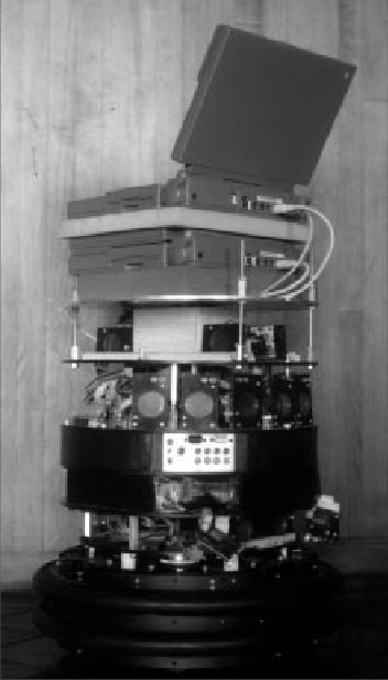
Dervish, shown in Figure 5.20, includes a sonar arrangement custom-designed for the 1994 AAAI National Robot Contest. The environment in this contest consisted of a rectilinear indoor office space filled with real office furniture as obstacles. Traditional sonars are ar- ranged radially around the robot in a ring. Robots with such sensor configurations are sub- ject to both tripping over short objects below the ring and to decapitation by tall objects (such as ledges, shelves and tables) that are above the ring. Dervish’s answer to this challenge was to arrange one pair of sonars diagonally upward to detect ledges and other overhangs. In addition, the diagonal sonar pair also proved to ably detect tables, enabling the robot to avoid wandering underneath tall tables. The remaining sonars were clustered in sets of sonars, such that each individual transducer in the set would be at a slightly varied angle to minimize specularity. Finally, two sonars near the robot’s base were able to detect low obstacles such as paper cups on the floor.
We have already noted that the representation provided by the contest organizers was purely topological, noting the connectivity of hallways and rooms in the office environment. Thus, it would be appropriate to design Dervish’s perceptual system to detect matching perceptual events: the detection and passage of connections between hallways and offices.
This abstract perceptual system was implemented by viewing the trajectory of sonar strikes to the left and right sides of Dervish over time. Interestingly, this perceptual system would use time alone and no concept of encoder value in order to trigger perceptual events. Thus, for instance, when the robot detects a 7 to 17 cm indentation in the width of the hallway for more than one second continuously, a closed door sensory event is triggered. If the sonar strikes jump well beyond 17 cm for more than one second, an open door sensory event trig- gers.
Sonars have a notoriously problematic error mode known as specular reflection: when the sonar unit strikes a flat surface at a shallow angle, the sound may reflect coherently away from the transducer, resulting in a large overestimate of range. Dervish was able to filter such potential noise by tracking its approximate angle in the hallway and completely sup- pressing sensor events when its angle to the hallway parallel exceeded 9 degrees. Interest- ingly, this would result in a conservative perceptual system that would easily miss features because of this suppression mechanism, particularly when the hallway is crowded with ob- stacles that Dervish must negotiate. Once again, the conservative nature of the perceptual system, and in particular its tendency to issue false negatives, would point to a probabilistic solution to the localization problem so that a complete trajectory of perceptual inputs could be considered.
Dervish’s environment representation was a classical topological map, identical in abstrac- tion and information to the map provided by the contest organizers. Figure 5.21 depicts a geometric representation of a typical office environment and the topological map for the same office environment. One can place nodes at each intersection and in each room, re- sulting in the case of figure 5.21 with four nodes total.
Once again, though, it is crucial that one maximize the information content of the represen- tation based on the available percepts. This means reformulating the standard topological graph shown in Figure 5.21 so that transitions into and out of intersections may both be used for position updates. Figure 5.22 shows a modification of the topological map in which just this step has been taken. In this case, note that there are 7 nodes in contrast to 4. In order to represent a specific belief state, Dervish associated with each topological node n a probability that the robot is at a physical position within the boundaries of n: p(r = n) . t As will become clear below, the probabilistic update used by Dervish was approximate, therefore technically one should refer to the resulting values as likelihoods rather than prob- abilities.
The perception update process for Dervish functions precisely as in Equation (5.21). Per- ceptual events are generated asynchronously, each time the feature extractor is able to rec- ognize a large-scale feature (e.g. doorway, intersection) based on recent ultrasonic values. Each perceptual event consists of a percept-pair (a feature on one side of the robot or two features on both sides).
| Wall | Closed Door | Open Door | Open Hallway | Foyer | |
| Nothing Detected | 0.70 | 0.40 | 0.05 | 0.001 | 0.30 |
| Closed Door Detected | 0.30 | 0.60 | 0 | 0 | 0.05 |
| Open Door Detected | 0 | 0 | 0.90 | 0.10 | 0.15 |
| Closed Hallway Detected | 0 | 0 | 0.001 | 0.90 | 0.5 |
Given a specific percept pair i, Equation (5.21) enables the likelihood of each possible po- sition n to be updated using the formula:
|
|
(1.8) |
The value of p(n) is already available from the current belief state of Dervish, and so the challenge lies in computing p(i|n). The key simplification for Dervish is based upon the re- alization that, because the feature extraction system only extracts 4 total features and be- cause a node contains (on a single side) one of 5 total features, every possible combination of node type and extracted feature can be represented in a 4 x 5 table. Dervish’s certainty matrix (show in Table 5.1) is just this lookup table. Dervish makes the simplifying assumption that the performance of the feature detector (i.e. the probability that it is correct) is only a function of the feature extracted and the actual feature in the node. With this assumption in hand, we can populate the certainty matrix with confidence estimates for each possible pairing of perception and node type. For each of the five world fea- tures that the robot can encounter (wall, closed door, open door, open hallway and foyer) this matrix assigns a likelihood for each of the three one-sided percepts that the sensory sys- tem can issue. In addition, this matrix assigns a likelihood that the sensory system will fail to issue a perceptual event altogether (nothing detected).
For example, using the specific values in Table 5.1, if Dervish is next to an open hallway, the likelihood of mistakenly recognizing it as an open door is 0.10. This means that for any node n that is of type Open Hallway and for the sensor value i=Open door, p(i|n) = 0.10. Together with a specific topological map, the certainty matrix enables straightforward com- putation of p(i|n) during the perception update process.
For Dervish’s particular sensory suite and for any specific environment it intends to navi- gate, humans generate a specific certainty matrix that loosely represents its perceptual con- fidence, along with a global measure for the probability that any given door will be closed versus opened in the real world.
Recall that Dervish has no encoders and that perceptual events are triggered asynchronously by the feature extraction processes. Therefore, Dervish has no action update step as depicted by Equation (5.22). When the robot does detect a perceptual event, multiple perception up- date steps will need to be performed in order to update the likelihood of every possible robot position given Dervish’s former belief state. This is because there is often a chance that the robot has traveled multiple topological nodes since its previous perceptual event (i.e. false negative errors). Formally, the perception update formula for Dervish is in reality a combi- nation of the general form of action update and perception update. The likelihood of posi- tion n given perceptual event i is calculated as in Equation (5.22):
|
|
(1.9) |
The value of p(n’ ) denotes the likelihood of Dervish being at position n’ as represented by Dervish’s former belief state. The temporal subscript t-i is used in lieu of t-1 because for each possible position n’ the discrete topological distance from n’ to n can vary depending on the specific topological map. The calculation of p(n n’ , i ) is performed by multi- tt-it plying the probability of generating perceptual event i at position n by the probability of hav- ing failed to generate perceptual events at all nodes between n’ and n:
For example (figure 5.23), suppose that the robot has only two nonzero nodes in its belief state, 1-2, 2-3, with likelihoods associated with each possible position: p(1-2) = 1.0 and p(2-3) = 0.2. For simplicity assume the robot is facing East with certainty. Note that the likelihoods for nodes 1-2 and 2-3 do not sum to 1.0. These values are not formal probabil- ities, and so computational effort is minimized in Dervish by avoiding normalization alto- gether. Now suppose that a perceptual event is generated: the robot detects an open hallway on its left and an open door on its right simultaneously. State 2-3 will progress potentially to states 3, 3-4 and 4. But states 3 and 3-4 can be elimi- nated because the likelihood of detecting an open door when there is only wall is zero. The likelihood of reaching state 4 is the product of the initial likelihood for state 2-3, 0.2, the like- lihood of not detecting anything at node 3, (a), and the likelihood of detecting a hallway on the left and a door on the right at node 4, (b). Note that we assume the likelihood of detecting nothing at node 3-4 is 1.0 (a simplifying approximation). (a) occurs only if Dervish fails to detect the door on its left at node 3 (either closed or open), [(0.6)(0.4) + (1-0.6)(0.05)], and correctly detects nothing on its right, 0.7. (b) occurs if Dervish correctly identifies the open hallway on its left at node 4, 0.90, and mis- takes the right hallway for an open door, 0.10. The final formula, (0.2)[(0.6)(0.4)+(0.4)(0.05)](0.7)[(0.9)(0.1)], yields a likelihood of 0.003 for state 4. This is a partial result for p(4) following from the prior belief state node 2-3. Turning to the other node in Dervish’s prior belief state, 1-2 will potentially progress to states 2, 2-3, 3, 3-4 and 4. Again, states 2-3, 3 and 3-4 can all be eliminated since the like- lihood of detecting an open door when a wall is present is zero. The likelihood of state 2 is the product of the prior likelihood for state 1-2, (1.0), the likelihood of detecting the door on the right as an open door, [(0.6)(0) + (0.4)(0.9)], and the likelihood of correctly detecting an open hallway to the left, 0.9. The likelihood for being at state 2 is then (1.0)(0.4)(0.9)(0.9) = 0.3. In addition, 1-2 progresses to state 4 with a certainty factor of -6 4.3 10 , which is added to the certainty factor above to bring the total for state 4 to 0.00328. Dervish would therefore track the new belief state to be 2, 4, assigning a very high likelihood to position 2 and a low likelihood to position 4. Empirically, Dervish’s map representation and localization system have proven to be suffi- cient for navigation of four indoor office environments: the artificial office environment cre- ated explicitly for the 1994 National Conference on Artificial Intelligence; the psychology department, the history department and the computer science department at Stanford Uni- versity. All of these experiments were run while providing Dervish with no notion of the distance between adjacent nodes in its topological map. It is a demonstration of the power of probabilistic localization that, in spite of the tremendous lack of action and encoder infor- mation, the robot is able to navigate several real-world office buildings successfully.
One open question remains with respect to Dervish’s localization system. Dervish was not just a localizer but also a navigator. As with all multiple hypothesis systems, one must ask the question, how does the robot decide how to move, given that it has multiple possible ro- bot positions in its representation? The technique employed by Dervish is a most common technique in the AMR ics field: plan the robot’s actions by assuming that the robot’s actual position is its most likely node in the belief state. Generally, the most likely position is a good measure of the robot’s actual world position. However, this technique has short- comings when the highest and second highest most likely positions have similar values. In the case of Dervish, it nonetheless goes with the highest likelihood position at all times, save at one critical juncture. The robot’s goal is to enter a target room and remain there. There- fore, from the point of view of its goal, it is critical that it finish navigating only when the robot has strong confidence in being at the correct final location. In this particular case, Der- vish’s execution module refuses to enter a room if the gap between the most likely position and the second likeliest position is below a preset threshold. In such a case, Dervish will actively plan a path that causes it to move further down the hallway in an attempt to collect more sensor data and thereby increase the relative likelihood of one position in the belief state. Although computationally unattractive, one can go further, imagining a planning system for robots such as Dervish for which one specifies a goal belief state rather than a goal position. The robot can then reason and plan in order to achieve a goal confidence level, thus explic- itly taking into account not only robot position but also the measured likelihood of each po- sition. An example of just such a procedure is the Sensory Uncertainty Field of Latombe [90], in which the robot must find a trajectory that reaches its goal while maximizing its lo- calization confidence enroute.
1.6.3 Kalman Filter Localisation
The Markov localization model can represent any probability density function over robot
position. This approach is very general but, due to its generality, inefficient. A successful alternative is to use a more compact representation of a specific class of probability densi- ties. The Kalman filter does just this, and is an optimal recursive data processing algorithm. It incorporates all information, regardless of precision, to estimate the current value of the variable of interest. A comprehensive introduction can be found in [46] and a more detailed treatment is presented in [28]. Figure 5.26 depicts the a general scheme of Kalman filter estimation, where the system has a control signal and system error sources as inputs. A measuring device enables measuring some system states with errors. The Kalman filter is a mathematical mechanism for produc- ing an optimal estimate of the system state based on the knowledge of the system and the measuring device, the description of the system noise and measurement errors and the un- certainty in the dynamics models. Thus the Kalman filter fuses sensor signals and system knowledge in an optimal way. Optimality depends on the criteria chosen to evaluate the per- formance and on the assumptions. Within the Kalman filter theory the system is assumed to be linear and white with Gaussian noise. As we have discussed earlier, the assumption of Gaussian error is invalid for our AMR applications but, nevertheless, the results are extremely useful. In other engineering disciplines, the Gaussian error assumption has in some cases been shown to be quite accurate [46]. We begin with a subsection that introduces Kalman filter theory, then we present an appli- cation of that theory to the problem of AMR localization. Finally, the third subsec- tion will present a case study of a AMR that navigates indoor spaces by virtue of Kalman filter localization.
A Gentle Introduction to Kalman Filter Theory
The
After presenting this static case, we can introduce dynamic prediction readily.
Static
Estimation
Let
us
assume
we
have
taken
two
-
one with an ultrasonic range sensor at time , and
-
one with a more precise laser range sensor at time .
Based on each measurement we are able to estimate the robot’s position.
Such an estimate derived from the first sensor measurements is and the estimate of position based on the second measurement is .
As
we
know
each
measurement
can
be
inaccurate,
we
wish
to
So
now
we
have
two
How do we fuse these data to get the best estimate for the robot position?
We are assuming that there was no robot motion between time and time , and therefore we can directly apply the same weighted least square technique:
|
|
(1.13) |
with being the weight of measurement . To find the minimum error we set the derivative i of S equal to zero. which gives us:
|
|
(1.14) |
Dynamic Estimation Following our previous model, we will now consider a robot which moves between successive sensor measurements. Suppose that the motion of the robot between times and is described by the velocity and the noise which represents the uncertainty of the actual velocity:
|
|
(1.15) |
If we now start at time , knowing the variance of the robot position at this time and knowing the variance of the motion, we obtain for the time just when the measurement is taken:
Kalman Filter Localisation
The
Kalman
filter
is
an
optimal
and
efficient
Application of the Kalman filter to localisation requires posing the robot localisation problem as a sensor fusion problem.
Recall
that
the
basic
probabilistic
update
of
robot
belief
state
can
be
segmented
into
two
-
perception update, and
-
action update
The fundamental difference between the Kalman filter approach and Markov localisation approach lies in the perception update process.
In
Markov
localisation,
the
entire
perception
In
some
cases,
the
perception
is
abstract,
having
been
produced
by
a
feature
extraction
mechanism.
By
contrast,
perception
update
using
a
Kalman
filter
is
a
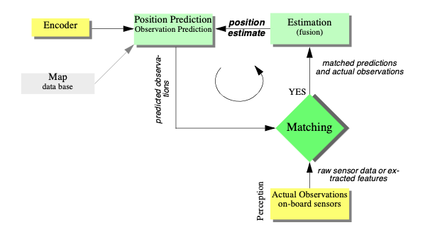
The
first
step
is
action
update
or
position
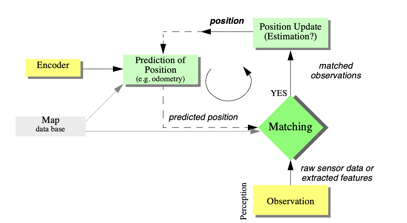
prediction,
the
straightforward
application
of
a
Gaussian
error
motion
model
to
the
robot’s
measured
encoder
travel.
The
robot
then
collects
actual
sensor
data
and
extracts
appropriate
features
1.7 Other Examples of Localisation Methods
Markov localisation and Kalman filter localisation have been two extremely popular strat- egies for research AMR systems navigating indoor environments. They have strong formal bases and therefore well-defined behavior. But there are a large number of other lo- calisation techniques that have been used with varying degrees of success on commercial and research AMR platforms. We will not explore the space of all localisation sys- tems in detail. Refer to surveys such as [4] for such information. There are, however, several categories of localisation techniques that deserve mention. Not surprisingly, many implementations of these techniques in commercial robotics employ modifications of the robot’s environment, something that the Markov localisation and Kal- man filter localisation communities eschew. In the following sections, we briefly identify the general strategy incorporated by each category and reference example systems, includ- ing as appropriate those that modify the environment and those that function without envi- ronmental modification.
1.7.1 Landmark-based Navigation
Landmarks are generally defined as
The control system for a landmark-based navigator consists of two
-
When a landmark is in view, the robot localizes frequently and accurately, using action update and perception update to
track its position without cumulative error . -
when the robot is in no landmark “zone”, then only action update occurs, and the robot accumulates position uncertainty until the next landmark enters the robot’s field of view.
The robot is thus effectively dead-reckoning from landmark zone to landmark zone. This in turn means the robot must consult its map carefully, ensuring that each motion between landmarks is sufficiently short, given its motion model, that it will be able to localize successful upon reaching the next landmark.
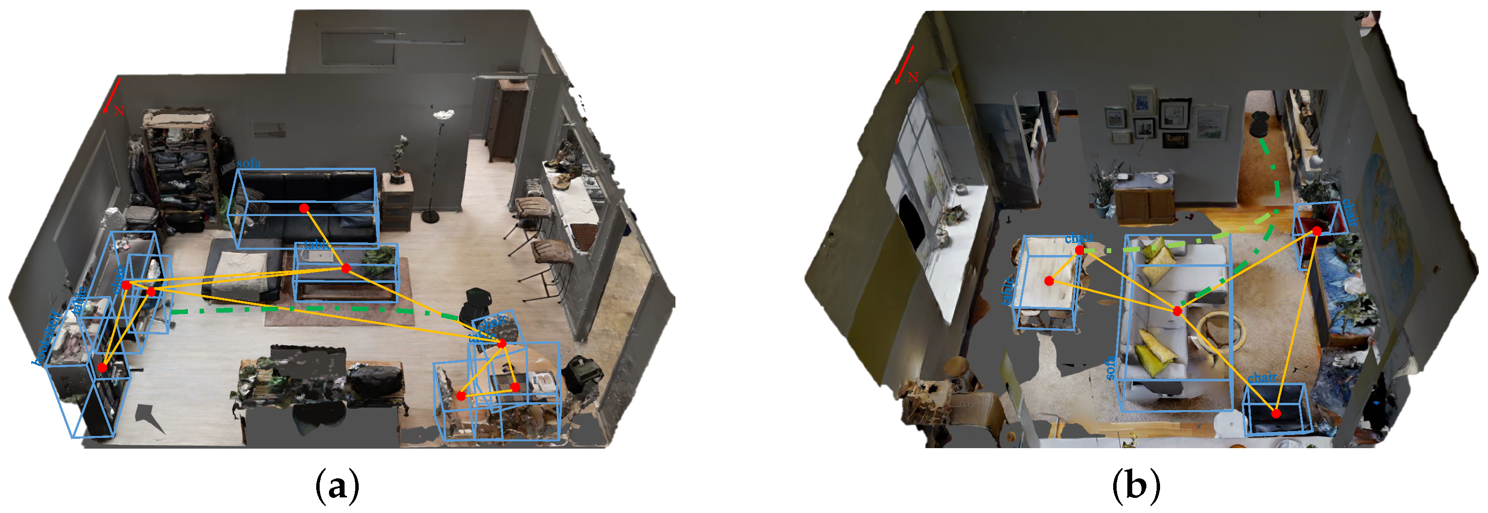
Fig. 1.12 shows one instantiating of landmark-based localisation. The particular shape of the landmarks enables reliable and accurate pose estimation by the robot, which must travel using dead reckoning between the landmarks.
One key advantage of the landmark-based navigation approach is that a strong formal theory has been developed for this general system architecture [113]. In this work, the authors have shown precise assumptions and conditions which, when satisfied, guarantee that the robot will always be able to localize successfully. This work also led to a real-world demonstration of landmark-based localisation. Standard sheets of paper were placed on the ceiling of the Robotics Laboratory at Stanford University, each with a unique checkerboard pattern. A Nomadics 200 AMR was fitted with a monochrome CCD camera aimed vertically up at the ceiling. By recognizing the paper landmarks, which were placed approximately 2 meters apart, the robot was able to localize to within several centimeters, then move using dead-reckoning to another landmark zone.
The primary disadvantage of landmark-based navigation is that in general
1.7.2 Globally Unique Localisation
The landmark-based navigation approach makes a strong general assumption:
when the landmark is in the robot’s field of view, localisation is essentially perfect.
One way to reach the near perfect AMR localisation is to effectively enable such an assumption to be valid wherever the robot is located. It would be revolutionary the robot’s sensors immediately identified its particular location, uniquely, and repeatedly.
Such a strategy for localisation is surely aggressive, but the question of whether it can be done is primarily a question of sensor technology software. Clearly, such a localisation system would need to use a sensor which collects a very large amount of information.
Since vision does indeed collect far more information than other sensors, it has been used as the sensor of choice in research towards globally unique localisation.
If humans were able to look at an individual picture and identify the robot’s location in a well-known environment, then one could argue that the information for globally unique localisation does exist within the picture. It must simply be interpreted correctly.
One such approach has been attempted by several researchers and involves constructing one or more image histograms to represent the information content of an image stably (see for example Figure 4.51 and Section 4.3.2.2). A robot using such an image histogramming system has been shown to uniquely identify individual rooms in an office building as well as individual sidewalks in an outdoor environment. However, such a system is highly sensitive to external illumination and provides only a level of localisation resolution equal to the visual footprint of the camera optics.
The Angular histogram depicted in Figure 5.37 is another example in which the robot’s sensor values are transformed into an identifier of location. However, due to the limited information content of sonar ranging strikes, it is likely that two places in the robot’s environment may have angular histograms that are too similar to be differentiated successfully.
One way of attempting to gather sufficient sonar information for global localisation is to allow the robot time to gather a large amount of sonar data into a local evidence grid (i.e. occupancy grid) first, then match the local evidence grid with a global metric map of the environment. In [115] the researchers demonstrate such a system as able to localize on-thefly even as significant changes are made to the environment, degrading the fidelity of the map. Most interesting is that the local evidence grid represents information well enough that it can be used to correct and update the map over time, thereby leading to a localisation system that provides corrective feedback to the environment representation directly. This is similar in spirit to the idea of taking rejected observed features in the Kalman filter localisation algorithm and using them to create new features in the map.
A most promising, new method for globally unique localisation is called Mosaic-based localisation [114]. This fascinating approach takes advantage of an environmental feature that is rarely used by AMR s: fine-grained floor texture. This method succeeds primarily because of the recent ubiquity of very fast processors, very fast cameras and very large storage media.
The robot is fitted with a high-quality high-speed CCD camera pointed toward the floor, ideally situated between the robot’s wheels and illuminated by a specialized light pattern off the camera axis to enhance floor texture. The robot begins by collecting images of the entire floor in the robot’s workspace using this camera. Of course the memory requirements are significant, requiring a 10GB drive in order to store the complete image library of a 300 x 300 meter area. Once the complete image mosaic is stored, the robot can travel any trajectory on the floor while tracking its own position without difficulty. Localisation is performed by simply re cording one image, performing action update, then performing perception update by matching the image to the mosaic database using simple techniques based on image database matching. The resulting performance has been impressive: such a robot has been shown to localize repeatedly with 1mm precision while moving at 25 km/hr. The key advantage of globally unique localisation is that, when these systems function correctly, they greatly simplify robot navigation. The robot can move to any point and will always be assured of localizing by collecting a sensor scan. But the main disadvantage of globally unique localisation is that it is likely that this method will never offer a complete solution to the localisation problem. There will always be cases where local sensory information is truly ambiguous and, therefore, globally unique localisa- tion using only current sensor information is unlikely to succeed. Humans often have excel- lent local positioning systems, particularly in non-repeating and well-known environments such as their homes. However, there are a number of environments in which such immediate localisation is challenging even for humans: consider hedge mazes and large new office buildings with repeating halls that are identical. Indeed, the mosaic-based localisation pro- totype described above encountered such a problem in its first implementation. The floor of the factory floor had been freshly painted and was thus devoid of sufficient micro-fractures to generate texture for correlation. Their solution was to modify the environment after all, painting random texture onto the factory floor.
1.7.3 Positioning Beacon systems
With most beacon systems, the design depicted depends foremost upon geometric principles to effect localisation. In this case the robots must know the positions of the two pinger units in the global coordinate frame in order to localize themselves to the global coordinate frame. A popular type of beacon system in industrial robotic applications is depicted in Figure 5.39. In this case beacons are retroreflective markers that can be easily detected by a AMR based on their reflection of energy back to the robot. Given known positions for the optical retroreflectors, a AMR can identify its position whenever it has three such beacons in sight simultaneously. Of course, a robot with encoders can localize over time as well, and does not need to measure its angle to all three beacons at the same instant. The advantage of such beacon-based systems is usually extremely high engineered reliabil- ity. By the same token, significant engineering usually surrounds the installation of such a system in a specific commercial setting. Therefore, moving the robot to a different factory floor will be both time-consuming and expensive. Usually, even changing the routes used by the robot will require serious re-engineering.
1.7.4 Route-Based Localisation
Even
more
reliable
than
beacon-based
systems
are
route-based
localisation
strategies.
In
this
case,
the
route
of
the
robot
is
explicitly
marked
so
that
it
can
determine
its
position,
not
relative
to
some
global
coordinate
frame,
but
relative
to
the
specific
path
it
is
allowed
to
travel.
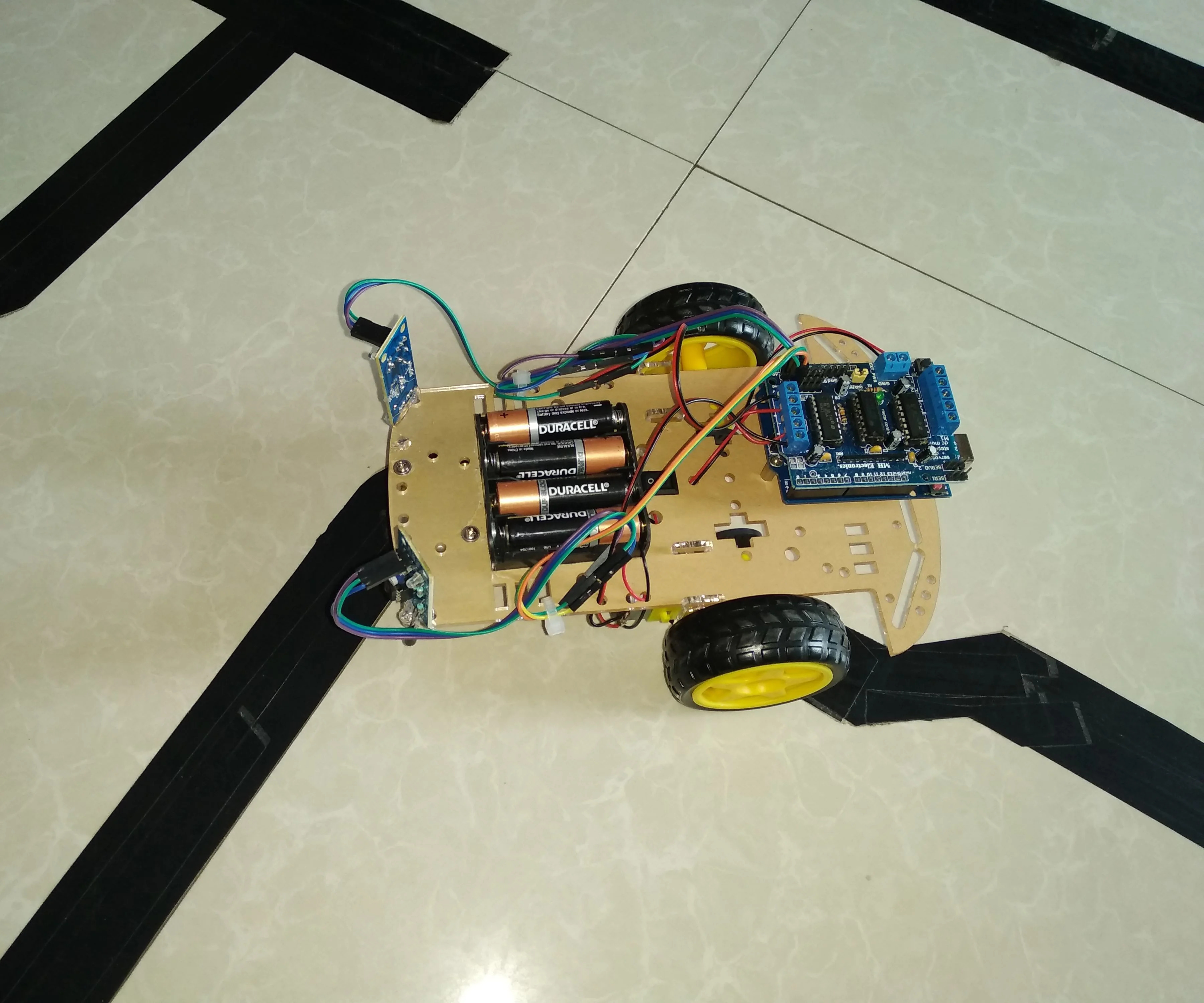
In all cases, one is effectively creating a railway system, except the railway system is somewhat more flexible and certainly more human-friendly actual rail.
For example, high UV-reflective, optically transparent paint can mark the route such that only the robot, using a specialized sensor, easily detects it. Alternatively, a guide wire buried underneath the hall can be detected using inductive coils located on the robot chassis.
In all such cases, the robot localisation problem is effectively trivialized by forcing the robot to always follow a prescribed path.
While this may remove the
the robot is much more inflexible give such localisation means, and therefore any change to the robot’s behavior requires significant engineering and time.
1.8 Building Maps
Humans are excellent navigators due to their remarkable ability to build cognitive maps [27] which form the basis of spatial memory [28], [29]. However, when it comes to AMR , we unfortunately need to be more hands on.
All of the localisation strategies we have discussed previously require active human effort to install the robot into a space. Artificial environmental modifications may be necessary to reduce ambiguity [30]. Even if this is not so, a map of the environment must be created for the robot.
But a robot which localizes successfully has the right sensors for detecting the environment, and so the robot ought to build its own map.
This ambition goes to the heart of AMR . In prose, we can express our eventual goal as follows:
Starting from an arbitrary initial point, a AMR should be able to autonomously explore the environment with its on-board sensors, gain knowledge about it, interpret the scene, build an appropriate map and localize itself relative to this map.
While
we
have
system
which
allows
certain
level
of
intelligence
to
robots,
most
applications
require
a
connected
network
or
a
central
node
to
achieve
any
autonomous
action [31], [32].
Accomplishing
this
goal
purely
using
internal
components
in
a
robust
is
probably
years
away,
but
an
important
sub-goal
is
the
invention
of
techniques
for
autonomous
creation
and
modification
of
an
environment
map.
Of
course
a
AMR
’s
sensors
have
only
limited
range,
and
so
it
must
physically
explore
its
environment
to
build
such
a
map.
So,
the
robot
must
not
only
create
a
map
but
it
must
do
so
while
moving
and
localizing
to
explore
the
environment.
This
is
often
called
the
Simultaneous
Localisation
and
Mapping
(SLAM)
problem,
The reason why SLAM is difficult is born precisely from the interaction between the robot’s position updates as it localises and its mapping actions. If a AMR updates its position based on an observation of an imprecisely known feature, the resulting position estimate becomes correlated with the feature location estimate. Similarly, the map becomes correlated with the position estimate if an observation taken from an imprecisely known position is used to update or add a feature to the map.
For localisation the robot needs to know where the features are whereas for map building the robot needs to know where it is on the map.
The only path to a complete and optimal solution to this joint problem is to consider all the correlations between between position estimation and feature location estimation. Such cross-correlated maps are called stochastic maps [34]. Unfortunately, implementing such an optimal solution is computationally prohibitive.
1.8.1 Stochastic Map Technique
Fig. 1.15 shows a general schematic incorporating map building and maintenance into the standard localisation loop depicted by Figure (5.29) during discussion of Kalman filter localisation [9]. The added arcs represent the additional flow of information that occurs when there is an imperfect match between observations and measurement predictions.
Unexpected observations will affect the creation of new features in the map whereas unobserved measurement predictions will affect the removal of features from the map. As discussed earlier, each specific prediction or observation has an unknown exact value and so it is represented by a distribution. The uncertainties of all of these quantities must be considered throughout this process.
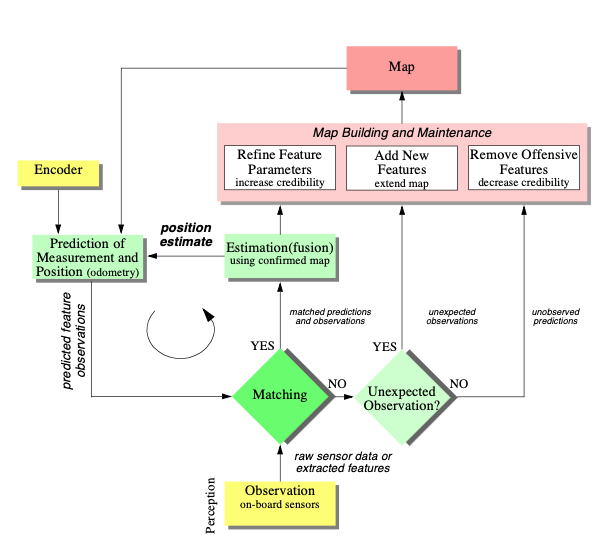
The new type of map we are creating not only has features in it as did previous maps, but it also has varying degrees of probability that each feature is indeed part of the environment.
We represent this new map
with a
set
of probabilistic feature locations
, each with the covariance matrix
and an associated
The purpose of is to quantify the belief in the existence of the feature in the environment (see Fig. (5.41)):
|
|
(1.19) |
In contrast to the map used for Kalman filter localisation previously, the map
is
NOT
assumed to be
Similar to Kalman filter localisation, the matching steps has three
-
matched prediction and observations,
-
unexpected observations, and
-
unobserved predictions
Localisation, or the position update of the robot, proceeds as before. However, the map is also updated now, using all three outcomes and complete propagation of all the correllated uncertainties.
The interesting concept in this modelling is the
How should the robot’s failure to match observed features to a particular map feature reduce that map feature’s credibility?
How should the robot’s success at matching a mapped feature increase the chance that the mapped feature is “correct?”
As an example, in [35] the following function is proposed for calculating credibility:
|
|
(1.20) |
where
and
define the
This forces us to use a stochastic map, in which all cross-correlations must be updated in each cycle.
The stochastic map consists of a stacked system state vector:
|
|
(1.21) |
and a system state covariance matrix:
|
|
(1.22) |
where the index r stands for the robot and the index i = 1 to n for the features in the map.
In contrast to localization based on an a priori accurate map, in the case of a stochastic map the cross-correlations must be maintained and updated as the robot is performing automatic map-building. During each localization cycle, the cross-correlations robot-to-feature and feature-to-robot are also updated. In short, this optimal approach requires every value in the map to depend on every other value, and therein lies the reason that such a complete solution to the automatic mapping problem is beyond the reach of even today’s computational resources.
1.8.2 Other Mapping Techniques
The AMR research community has spent significant research effort on the problem of automatic mapping, and has demonstrating working systems in many environments without having solved the complete stochastic map problem described earlier.
This field of AMR research is extremely large, and this Lecture Book will NOT present a comprehensive survey of the field
Instead, let’s look at the two
Cyclic Environments
Possibly the single hardest challenge for automatic mapping to be conquered is to correctly map cyclic environments. The problem is simple:
Given
an
environment
which
has
one
or
more
loops
or
cycles,
This problem is hard because of the fundamental behavior of automatic mapping systems:
The maps they create are not perfect.
And, given any local imperfection, accumulating such imperfections over time can lead to arbitrarily large global errors between a map, at the macro level, and the real world, as shown in Fig. 1.16 .
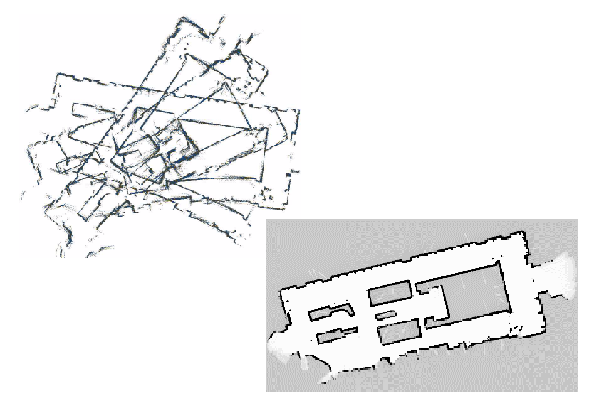
Such global error is usually irrelevant for
AMR
localisation and navigation. After all, a warped map will still serve the robot
perfectly well
With the recent popularity of metric maps such as fixed decomposition grid representations, the cycle detection strategy is not as straightforward. Two important features are found in most autonomous mapping systems that claim to solve the cycle detection problem:
-
First, as with many recent systems, these mobile robots tend to accumulate recent perceptual history to
create small-scale local sub-maps [37]. In this approach, each sub-map is treated as a singular sensor during the robot’s position update. The advantage of this approach is two-fold.-
As odometry is relatively accurate over small distances, the relative registration of features and raw sensor strikes in a local sub-map will be quite accurate.
-
The robot will have created a virtual sensor system with a significantly larger horizon than its actual sensor system’s range. In a sense, this strategy at the very least defers the problem of very large cyclic environments by increasing the map scale that can be handled well by the robot.
-
-
The second recent technique for dealing with cycle environments is in fact a
return to the topological representation . Some recent automatic mapping systems will attempt to identify cycles by associating a topology with the set of metric sub-maps, explicitly identifying the loops first at the topological level.
One could certainly imagine other augmentations based on known topological methods.
For example, the globally unique localisation methods described previously could be used to identify topological correctness.
Dynamic Environments
A second challenge extends NOT just to existing autonomous mapping solutions but even to the basic execution of the stochastic map approach.
All previously mentioned strategies tend to assume the environment is either
However, for many practical applications, this assumption is lacking at best. In the case of wide-open spaces that are popular gathering places for humans, there is rapid change in the freespace and a vast majority of sensor strikes represent detection of the transient humans rather than fixed surfaces such as the perimeter wall.
Another class of dynamic environments are spaces such as factory floors and warehouses, where the objects being stored redefine the topology of the pathways on a day-to-day basis as shipments are moved in and out.
In
all
such
dynamic
environments,
an
automatic
mapping
system
should
capture
the
salient
The
subject
of
For example, in the case of stochastic mapping using the credibility factor mechanism, the credibility equation can continue to provide feedback regarding the probability of existence of various mapped features after the initial map creation process is ostensibly complete. Therefore, a mapping system can become a map-modifying system by simply continuing to operate.
This is most effective, of course, if the mapping system is real-time and incremental.
If map construction requires off-line global optimisation, then the desire to make small-grained, incremental adjustments to the map is more difficult to satisfy.
Earlier we stated that a mapping system should capture only the salient objects detected by its sensors. One common argument for handling the detection of, for instance, humans in the environment is that mechanisms such as serve to be mapped in the first place.
The general solution to the problem of detecting salient features, however, requires a solution to the perception problem in general. When a robot’s sensor system can reliably detect the difference between a wall and a human, using for example a vision system, then the problem of mapping in dynamic environments will become significantly more straightforward.
We have discussed just two important considerations for automatic mapping. There is still a great deal of research activity focusing on the general map building and localisation problem. This field is certain to produce significant new results in the next several years, and as the perceptual power of robots improves we expect the payoff to be greatest here.
ttt
Information : DARPA Grand Challenge
A prize competition for American autonomous vehicles, funded by the Defense Advanced Research Projects Agency (DARPA). The goal of the challenge is too further DARPA’s mission to sponsor revolutionary, high-payoff research that bridges the gap between fundamental discoveries and military use. The initial DARPA Grand Challenge in 2004 was created to spur the development of technologies needed to create the first fully autonomous ground vehicles capable of completing a substantial off-road course within a limited time. The third event, the DARPA Urban Challenge in 2007, extended the initial Challenge to autonomous operation in a mock urban environment. The 2012 DARPA Robotics Challenge, focused on autonomous emergency-maintenance robots, and new Challenges are still being conceived. The DARPA Subterranean Challenge was tasked with building robotic teams to autonomously map, navigate, and search subterranean environments. Such teams could be useful in exploring hazardous areas and in search and rescue.