2
Perception
2.1 Introduction
One
of
the
most
important
tasks
of
an
AMR
is
to
acquire
knowledge
about
its
environment.
In
this
chapter
we
present
the
most
common
sensors
used
in
AMR
and
then
discuss
strategies
for
2.1.1 Sensors for Mobile Robotics
There is a wide variety of sensors used in
AMR
s (Fig. 4.1). Some are used to measure simple values like the
internal temperature of a robot’s electronics or the rotational speed of the motors in its wheels or actuators.
Other, more sophisticated sensors can be used to acquire information about the robot’s environment or even to
directly measure a robot’s global position. Here, we focus primarily on sensors used to extract information about
the robot’s environment. Because a
AMR
moves around, it will frequently encounter
2.1.2 Sensor Classification
We classify sensors using two
- Proprioceptive
-
sensors which measure values
internal to the robot.e.g., motor speed, wheel load, robot arm joint angles, battery voltage.
- Exteroceptive
-
sensors which measure information from the
robot’s environment ;e.g., distance measurements, light intensity, sound amplitude.
exteroceptive sensor measurements are interpreted by the robot to extract meaningful environmental features.
- Passive
-
sensors measure ambient environmental energy entering the sensor.
e.g., temperature probes, microphones and Charge Coupled Device (CCD) or CMOS cameras.
- Active
-
sensors emit energy into the environment, then measure the environmental reaction. Because active sensors can manage more controlled interactions with the environment, they often achieve superior performance. However, active sensing introduces several risks: the outbound energy may affect the very characteristics that the sensor is attempting to measure. Furthermore, an active sensor may suffer from interference between its signal and those beyond its control. For example, signals emitted by other nearby robots, or similar sensors on the same robot my influence the resulting measurements. Examples of active sensors include wheel quadrature encoders, ultrasonic sensors and laser rangefinders.
The sensor classes in Table (4.1) are arranged in ascending order of complexity and descending order of technological maturity. Tactile sensors and proprioceptive sensors are critical to virtually all mobile robots, and are well understood and easily implemented. Commercial quadrature encoders, for example, may be purchased as part of a gear-motor assembly used in a AMR . At the other extreme, visual interpretation by means of one or more CCD /CMOS cameras provides a broad array of potential functionalities, from obstacle avoidance and localisation to human face recognition. However, commercially available sensor units that provide visual functionalities are only now beginning to emerge
2.1.3 Characterising Sensor Performance
The sensors we describe in this chapter vary greatly in their performance characteristics. Some sensors provide extreme accuracy in well-controlled laboratory settings, but are overcome with error when subjected to real-world environmental variations. Other sensors provide narrow, high precision data in a wide variety settings. To quantify such performance characteristics, first we formally define the sensor performance terminology that will be valuable throughout the rest of this chapter.
Basic Sensor Response Ratings
A number of sensor characteristics can be rated
- Dynamic Range
-
Used to measure the spread between the lower and upper limits of inputs values to the sensor while maintaining normal sensor operation. Formally, the dynamic range is the ratio of the maximum input value to the minimum measurable input value. Because this raw ratio can be unwieldy, it is usually measured in Decibels, which is computed as ten times the common logarithm of the dynamic range. However, there is potential confusion in the calculation of Decibels, which are meant to measure the ratio between powers, such as Watts or Horsepower.
Suppose your sensor measures motor current and can register values from a minimum of 1 mA to 20 A . The dynamic range of this current sensor is defined as:
(2.1) Now suppose you have a voltage sensor that measures the voltage of your robot’s battery, measuring any value from 1 mV to 20 V . Voltage is NOT a unit of power, but the square of voltage is proportional to power. Therefore, we use 20 instead of 10:
(2.2) - Range
-
An important rating in AMR because often robot sensors operate in environments where they are frequently exposed to input values beyond their working range. In such cases, it is critical to understand how the sensor will respond. For example, an optical rangefinder will have a minimum operating range and can thus provide spurious data when measurements are taken with object closer than that minimum.
- Resolution
-
The minimum difference between two
(2) values that can be detected by a sensor. Usually, the lower limit of the dynamic range of a sensor is equal to its resolution. However, in the case of digital sensors, this is not necessarily so. For example, suppose that you have a sensor that measures voltage, performs an analogue-to-digital conversion and outputs the converted value as an 8-bit number linearly corresponding to between 0 and 5 Volts. If this sensor is truly linear, then it has total output values or a resolution of: - Linearity
-
is an important measure governing the behaviour of the sensor’s output signal as the input signal varies. A linear response indicates that if two
(2) inputs, say and result in the two outputs and , then for any values and , the following relation can be derived:This means that a plot of the sensor’s input/output response is simply a straight line.
- Bandwidth or Frequency
-
is used to measure the speed with which a sensor can provide a stream of readings. Formally, the number of measurements per second is defined as the sensor’s frequency in Hz . Because of the dynamics of moving through their environment, mobile robots often are limited in maximum speed by the bandwidth of their obstacle detection sensors. Thus increasing the bandwidth of ranging and vision-based sensors has been a high-priority goal in the robotics community.
In Situ Sensor Performance
The above sensor characteristics can be reasonably measured in a laboratory environment, with confident extrapolation to performance in real-world deployment. However, a number of important measures cannot be reliably acquired without deep understanding of the complex interaction between all environmental characteristics and the sensors in question. This is most relevant to the most sophisticated sensors, including active ranging sensors and visual interpretation sensors.
- Sensitivity
-
A measure of the degree to which an incremental change in the target input signal changes the output signal. Formally, sensitivity is the ratio of output change to input change. Unfortunately, however, the sensitivity of exteroceptive sensors is often confounded by undesirable sensitivity and performance coupling to other environmental parameters.
- Cross-Sensitivity
-
is the technical term for sensitivity to environmental parameters that are orthogonal to the target parameters for the sensor. For example, a flux-gate compass can demonstrate high sensitivity to magnetic north and is therefore of use for AMR navigation. However, the compass will also demonstrate high sensitivity to ferrous building materials, so much so that its cross-sensitivity often makes the sensor useless in some indoor environments. High cross-sensitivity of a sensor is generally undesirable, especially so when it cannot be modelled.
- Error
-
of a sensor is defined as the difference between the sensor’s output measurements and the true values being measured, within some specific operating context.
As an example, given a true value and a measured value , we can define error as:
- Accuracy
-
defined as the degree of conformity between the sensor’s measurement and the true value, and is often expressed as a proportion of the true value (e.g. 97.5% accuracy):
Of course, obtaining the ground truth ( ), can be difficult or impossible, and so establishing a confident characterisation of sensor accuracy can be problematic. Further, it is important to distinguish between two different sources of error:
-
Systematic errors are caused by factors or processes that can in theory be modelled. These errors are, therefore, deterministic.
2 2 Meaning, it’s value is not determined by a random process and therefore should, in theory, be predictable.Poor calibration of a laser rangefinder, un-modelled slope of a hallway floor and a bent stereo camera head due to an earlier collision are all possible causes of systematic sensor errors
-
Random errors cannot be predicted using a sophisticated model nor can they be mitigated with more precise sensor machinery. These errors can only be described in probabilistic terms (i.e. stochastic). Hue instability in a colour camera, spurious range-finding errors and black level noise in a camera are all examples of random errors.
-
- Precision
-
is often confused with accuracy, and now we have the tools to clearly distinguish these two terms. Intuitively, high precision relates to reproducibility of the sensor results. For example, one sensor taking multiple readings of the same environmental state has high precision if it produces the same output. In another example, multiple copies of this sensors taking readings of the same environmental state have high precision if their outputs agree. Precision does not, however, have any bearing on the accuracy of the sensor’s output with respect to the true value being measured. Suppose that the random error of a sensor is characterised by some mean value ( ) and a standard deviation ( ). The formal definition of precision is the ratio of the sensor’s output range to the standard deviation:
Only and NOT has impact on precision. In contrast mean error is directly proportional to overall sensor error and inversely proportional to sensor accuracy.
Characterising Error
Mobile robots depend heavily on
Of
course,
these
“objects”
surrounding
the
robot
are
all
detected
from
the
viewpoint
of
its
local
reference
frame.
Now
that
we
have
the
necessary
knowledge
on
the
fundamental
concepts
and
terminology,
we
can
now
describe
how
dramatically
the
sensor
error
of
an
AMR
Blurring of Systematical and Random Errors
Active ranging sensors tend to have failure modes which are triggered largely by specific relative positions of the sensor and environment targets.
For
example,
a
sonar
sensor
will
product
specular
reflections,
During motion of the robot, such relative angles occur at stochastic intervals. This is especially true in a
AMR
outfitted with a
ring of multiple sonars. The chances of one sonar entering this error mode during robot motion is high. From the perspective of
the moving robot, the sonar measurement error is a
If the robot’s static position causes a particular sonar to fail in this manner, the sonar will fail consistently and will tend to return precisely the same (and incorrect!) reading time after time. Once the robot is motionless, the error appears to be systematic and high precision.
The fundamental mechanism at work here is the cross-sensitivity of AMR sensors to robot pose and robot-environment dynamics.
The
models
for
such
cross-sensitivity
are
NOT
,
in
an
underlying
sense,
truly
random.
However,
these
physical
interrelationships
are
rarely
modelled
and
therefore,
from
the
point
of
view
of
an
incomplete
model,
the
errors
appear
random
during
motion
and
systematic
when
the
robot
is
at
rest.
Sonar
is
not
the
only
sensor
subject
to
this
blurring
of
systematic
and
random
error
modality.
Visual
interpretation
through
the
use
of
a
CCD
camera
is
also
highly
susceptible
to
robot
motion
and
position
because
of
camera
dependency
on
lighting.
The important point is to realise that, while systematic error and random error are well-defined in a controlled setting, the AMR can exhibit error characteristics that bridge the gap between deterministic and stochastic error mechanisms.
Multi-Modal Error Distributions
It is common to characterise the behaviour of a sensor’s random error in terms of a probability distribution over various output values. In general, one knows very little about the causes of random error and therefore several simplifying assumptions are commonly used. For example, we can assume that the error is zero-mean ( ), in that it symmetrically generates both positive and negative measurement error. We can go even further and assume that the probability density curve is Gaussian. Although we discuss the mathematics of this in detail later, it is important for now to recognise the fact that one frequently assumes symmetry as well as unimodal distribution. This means that measuring the correct value is most probable, and any measurement that is further away from the correct value is less likely than any measurement that is closer to the correct value. These are strong assumptions that enable powerful mathematical principles to be applied to AMR problems, but it is important to realise how wrong these assumptions usually are.
Consider,
for
example,
the
sonar
sensor
once
again.
When
ranging
an
object
that
reflects
the
sound
signal
well,
the
sonar
will
exhibit
high
accuracy,
and
will
induce
random
error
based
on
noise,
for
example,
in
the
timing
circuitry.
This
portion
of
its
sensor
behaviour
will
exhibit
error
characteristics
that
are
fairly
As
a
second
example,
consider
ranging
via
stereo
vision.
Once
again,
we
can
identify
two
2.1.4 Wheel and Motor Sensors
Wheel/motor sensors are devices use to measure the internal state and dynamics of a mobile robot. These sensors have vast applications outside of AMR and, as a result, AMR has enjoyed the benefits of high-quality, low-cost wheel and motor sensors which offer excellent resolution.
In the next part, we sample just one such sensor, the optical incremental encoder.
Optical Encoders
Optical incremental encoders have become the most popular device for measuring angular speed and position within a motor drive or at the shaft of a wheel or steering mechanism. In mobile robotics, encoders are used to control the position or speed of wheels and other mo- tor-driven joints. Because these sensors are proprioceptive, their estimate of position is best in the reference frame of the robot and, when applied to the problem of robot localisation, significant corrections are required as discussed in Chapter 5.
An optical encoder is basically a mechanical light chopper that produces a certain number of sine or square wave pulses for each shaft revolution. It consists of an illumination source, a fixed grating that masks the light, a rotor disc with a fine optical grid that rotates with the shaft, and fixed optical detectors. As the rotor moves, the amount of light striking the optical detectors varies based on the alignment of the fixed and moving gratings. In robotics, the resulting sine wave is transformed into a discrete square wave using a threshold to choose between light and dark states. Resolution is measured in Cycles Per Revolution (CPR). The minimum angular resolution can be readily computed from an encoder’s CPR rating. A typical encoder in AMR may have 2,000 CPR while the optical encoder industry can readily manufacture encoders with 10,000 CPR. In terms of required bandwidth, it is of course critical that the encoder be sufficiently fast to count at the shaft spin speeds that are expected. Industrial optical encoders present no bandwidth limitation to AMR applications. Usually in AMR the quadrature encoder is used. In this case, a second illumination and detector pair is placed 90ř shifted with respect to the original in terms of the rotor disc. The resulting twin square waves, shown in Fig. 4.2, provide significantly more information. The ordering of which square wave produces a rising edge first identifies the direction of rotation. Furthermore, the four detectability different states improve the resolution by a factor of four with no change to the rotor disc. Thus, a 2,000 CPR encoder in quadrature yields 8,000 counts. Further improvement is possible by retaining the sinusoidal wave measured by the optical detectors and performing sophisticated interpolation. Such methods, although rare in AMR , can yield 1000-fold improvements in resolution. As with most proprioceptive sensors, encoders are generally in the controlled environment of a AMR ’s internal structure, and so systematic error and cross-sensitivity can be engineered away. The accuracy of optical encoders is often assumed to be 100% and, although this may not entirely correct, any errors at the level of an optical encoder are dwarfed by errors downstream of the motor shaft.
Heading Sensors
Heading sensors can be proprioceptive (gyroscope, inclinometer) or exteroceptive (com- pass). They are used to determine the robots orientation and inclination. They allow us, to- gether with appropriate velocity information, to integrate the movement to a position estimate. This procedure, which has its roots in vessel and ship navigation, is called dead reckoning.
Compasses
The two most common modern sensors for measuring the direction of a magnetic field are the Hall Effect and Flux Gate compasses. Each has advantages and disadvantages, as described below. The Hall Effect describes the behaviour of electric potential in a semiconductor when in the presence of a magnetic field. When a constant current is applied across the length of a semi- conductor, there will be a voltage difference in the perpendicular direction, across the semi- conductor’s width, based on the relative orientation of the semiconductor to magnetic flux
lines. In addition, the sign of the voltage potential identifies the direction of the magnetic field. Thus, a single semiconductor provides a measurement of flux and direction along one dimension. Hall Effect digital compasses are popular in AMR , and contain two such semiconductors at right angles, providing two axes of magnetic field (thresholded) direction, thereby yielding one of 8 possible compass directions. The instruments are inexpensive but also suffer from a range of disadvantages. Resolution of a digital hall effect compass is poor. Internal sources of error include the nonlinearity of the basic sensor and systematic bias errors at the semiconductor level. The resulting circuitry must perform significant filtering, and this lowers the bandwidth of hall effect compasses to values that are slow in AMR terms. For example the hall effect compasses pictured in figure 4.3 needs 2.5 seconds to settle after a 90ř spin. The Flux Gate compass operates on a different principle. Two small coils are wound on fer- rite cores and are fixed perpendicular to one-another. When alternating current is activated in both coils, the magnetic field causes shifts in the phase depending upon its relative alignment with each coil. By measuring both phase shifts, the direction of the magnetic field in two dimensions can be computed. The flux-gate compass can accurately measure the strength of a magnetic field and has improved resolution and accuracy; however it is both larger and more expensive than a Hall Effect compass. Regardless of the type of compass used, a major drawback concerning the use of the Earth’s magnetic field for AMR applications involves disturbance of that magnetic field by other magnetic objects and man-made structures, as well as the bandwidth limitations of electronic compasses and their susceptibility to vibration. Particularly in indoor environments AMR applications have often avoided the use of compasses, although a compass can conceivably provide useful local orientation information indoors, even in the precense of steel structures.
Gyroscope
Gyroscopes are heading sensors which preserve their orientation in relation to a fixed refer- ence frame. Thus they provide an absolute measure for the heading of a mobile system. Gy- roscopes can be classified in two categories, mechanical gyroscopes and optical gyroscopes.
Mechanical Gyroscopes
The concept of a mechanical gyroscope relies on the inertial properties of a fast spinning rotor. The property of interest is known as the gyroscopic precession. If you try to rotate a fast spinning wheel around its vertical axis, you will feel a harsh reaction in the horizontal axis. This is due to the angular momentum associated with a spinning wheel and will keep the axis of the gyroscope inertially stable. The reactive torque and thus the tracking stability with the inertial frame are proportional to the spinning speed , the precession speed and the wheel’s inertia I.
By arranging a spinning wheel as seen in Figure 4.4, no torque can be transmitted from the outer pivot to the wheel axis. The spinning axis will therefore be space-stable (i.e. fixed in an inertial reference frame). Nevertheless, the remaining friction in the bearings of the gyro- axis introduce small torques, thus limiting the long term space stability and introducing small errors over time. A high quality mechanical gyroscope can cost up to $100,000 and has an angular drift of about 0.1ř in 6 hours. For navigation, the spinning axis has to be initially selected. If the spinning axis is aligned with the north-south meridian, the earth’s rotation has no effect on the gyro’s horizontal axis. If it points east-west, the horizontal axis reads the earth rotation. Rate gyros have the same basic arrangement as shown in Figure 4.4 but with a slight modification. The gimbals are restrained by a torsional spring with additional viscous damping. This enables the sensor to measure angular speeds instead of absolute orientation.
Optical Gyroscopes
Optical gyroscopes are a relatively new innovation. Commercial use began in the early 1980’s when they were first installed in aircraft. Optical gyroscopes are angular speed sen- sors that use two monochromatic light beams, or lasers, emitted from the same source in- stead of moving, mechanical parts. They work on the principle that the speed of light remains unchanged and, therefore, geometric change can cause light to take a varying amount of time to reach its destination. One laser beam is sent traveling clockwise through a fiber while the other travels counterclockwise. Because the laser traveling in the direction of rotation has a slightly shorter path, it will have a higher frequency. The difference in fre- quency of the two beams is a proportional to the angular velocity of the cylinder. New solid-state optical gyroscopes based on the same principle are build using microfabrication technology, thereby providing heading information with resolution and bandwidth far beyond the needs of mobile robotic applications. Bandwidth, for instance, can easily exceed 100KHz while resolution can be smaller than 0.0001ř/hr.
Ground Based Beacons
One elegant approach to solving the localization problem in AMR is to use active or passive beacons. Using the interaction of on-board sensors and the environmental bea- cons, the robot can identify its position precisely. Although the general intuition is identical to that of early human navigation beacons, such as stars, mountains and lighthouses, modern technology has enabled sensors to localize an outdoor robot with accuracies of better than 5 cm within areas that are kilometres in size.
In the following subsection, we describe one such beacon system, the Global Positioning System (GPS), which is extremely effective for outdoor ground-based and flying robots. In- door beacon systems have been generally less successful for a number of reasons. The ex- pense of environmental modification in an indoor setting is not amortized over an extremely large useful area, as it is for example in the case of GPS. Furthermore, indoor environments offer significant challenges not seen outdoors, including multipath and environment dynam- ics. A laser-based indoor beacon system, for example, must disambiguate the one true laser signal from possibly tens of other powerful signals that have reflected off of walls, smooth floors and doors. Confounding this, humans and other obstacles may be constantly changing the environment, for example occluding the one true path from the beacon to the robot. In commercial applications such as manufacturing plants, the environment can be carefully controlled to ensure success. In less structured indoor settings, beacons have nonetheless been used, and the problems are mitigated by careful beacon placement and the useful of passive sensing modalities.
Global Positioning System
The
Global
Positioning
System
(GPS)
was
initially
developed
for
military
use
but
is
now
freely
available
for
civilian
navigation.
There
are
at
least
24
operational
GPS
satellites
at
all
times.
The
satellites
orbit
every
12
hours
at
a
height
of
20.190km.
There
are
four
Each
satellite
continuously
transmits
data
which
indicates
its
location
and
the
current
time.
Therefore,
GPS
receivers
are
By
combining
information
regarding
the
arrival
time
and
instantaneous
location
of
four
In
theory,
such
triangulation
requires
only
three
It
is,
of
course,
mandatory
the
satellites
to
be
well
synchronised.
To
this
end,
they
are
updated
by
ground
stations
regularly
and
each
satellite
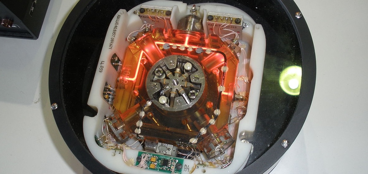
carries
on-board
atomic
clocks
The second point is that GPS satellites are merely an information source. They can be employed with various strategies in order to achieve dramatically different levels of localisation resolution. The basic strategy for GPS use, called pseudorange and described above, generally performs at a resolution of 15m. An extension of this method is differential GPS, which makes use of a second receiver that is static and at a known exact position. A number of errors can be corrected using this reference, and so resolution improves to the order of 1m or less. A disadvantage of this technique is that the stationary receiver must be installed, its location must be measured very carefully and of course the moving robot must be within ki- lometers of this static unit in order to benefit from the DGPS technique. A further improved strategy is to take into account the phase of the carrier signals of each received satellite transmission. There are two carriers, at 19cm and 24cm, therefore signif- icant improvements in precision are possible when the phase difference between multiple satellites is measured successfully. Such receivers can achieve 1cm resolution for point po- sitions and, with the use of multiple receivers as in DGPS, sub-1cm resolution. A final consideration for AMR applications is bandwidth. GPS will generally offer no better than 200 - 300ms latency, and so one can expect no better than 5Hz GPS updates. On a fast-moving AMR or flying robot, this can mean that local motion integration will be required for proper control due to GPS latency limitations.
2.2 Active Ranging
Active range sensors continue to be the most popular sensors used in AMR . Many ranging sensors have a low price point, and most importantly all ranging sensors provide easily interpreted outputs:
Direct measurements of distance from the robot to objects in its vicinity.
For obstacle detection and avoidance, most AMR rely heavily on active ranging sensors. But the local free-space information provided by range sensors can also be accumulated into representations beyond the robot’s current local reference frame. Therefore, active range sensors are also commonly found as part of the localisation and environmental modelling processes of AMR s.
It is only with the slow advent of successful visual interpretation competency that we can expect the class of active ranging sensors to gradually lose their primacy as the sensor class of choice among AMR engineers.
Below,
we
present
two
-
the ultrasonic sensor,
-
the laser rangefinder.
Continuing
onwards,
we
then
present
two
-
the optical triangulation sensor,
-
the structured light sensor.
Time-of-FLight Active Ranging
ToF
ranging
makes
use
of
the
where is the distance travelled usually round-trip ( m ), the speed of wave propagation ( ms − 1 ), and is the time it takes to travel ( s ).
It
is
important
to
point
out
the
propagation
speed
of
sound
is
approximately
0.3
mms
−
1
whereas
the
speed
of
an
electromagnetic
signal
is
0.3
mns
−
1
,
which
is
one
million
times
faster.
The
ToF
for
a
typical
distance,
say
3
m
,
is
10
ms
for
an
ultrasonic
system
but
only
10
ns
for
a
laser
rangefinder.
It
is
therefore
obvious
that
measuring
the
time
of
flight
with
electromagnetic
signals
is
more
technologically
challenging.
The quality of ToF range sensors depends mainly on the following:
-
Uncertainties in determining the exact time of arrival of the reflected signal,
-
Inaccuracies in the time of flight measurement, particularly with laser range sensors,
-
The dispersal cone of the transmitted beam mainly with ultrasonic range sensors
-
Interaction with the target (e.g., surface absorption, specular reflections)
-
Variation of propagation speed, and
-
The speed of the AMR and target (in the case of a dynamic target).
As discussed below, each type of ToF sensor is sensitive to a particular subset of the above list of factors.
2.2.1 The Ultrasonic Sensor
The
main
ethos
of
an
ultrasonic
The speed of sound in air is given by the following relation:
where
is
the
ratio
of
specific
heat,
is
the
gas
constant
(
Jmol
−
1
K
−
1
),
and
is
the
temperature
in
Kelvin
(
).
In
air,
at
standard
pressure,
and
20
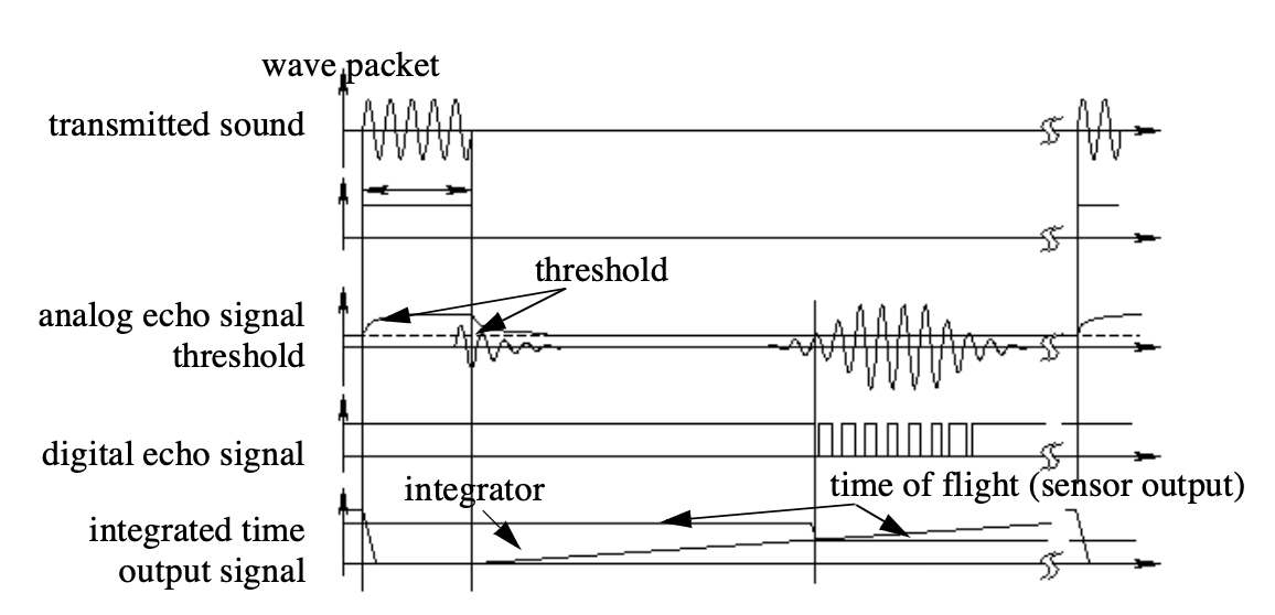
We can see the different signal output and input of an ultrasonic sensor in Fig. 2.5 .
First,
a
series
of
sound
pulses
are
emitted,
which
creates
the
wave
packet.
An
integrator
also
begins
to
This threshold is often decreasing in time, because the amplitude of the expected echo decreases over time based on dispersal as it travels longer.
But during transmission of the initial sound pulses and just afterwards, the threshold is set very high to suppress triggering the echo detector with the outgoing sound pulses. A transducer will continue to ring for up to several ms after the initial transmission, and this governs the blanking time of the sensor.
If, during the blanking time, the transmitted sound were to reflect off of an extremely close object and return to the ultrasonic sensor, it may fail to be detected.
However, once the blanking interval has passed, the system will detect any above-threshold reflected sound, triggering a digital signal and producing the distance measurement using the integrator value.
The ultrasonic wave typically has a frequency between 40 and 180 kHz and is usually generated by a piezo or electrostatic transducer. Often the same unit is used to measure the reflected signal, although the required blanking interval can be reduced through the use of separate output and input devices. Frequency can be used to select a useful range when choosing the appropriate ultrasonic sensor for a AMR . Lower frequencies correspond to a longer range, but with the disadvantage of longer post-transmission ringing and, therefore, the need for longer blanking intervals.
Most ultrasonic sensors used by AMR s have an effective range of roughly 12 cm to 5 metres. The published accuracy of commercial ultrasonic sensors varies between 98% and 99.1%. In AMR applications, specific implementations generally achieve a resolution of approximately 2 cm .
In
most
cases
one
may
want
a
narrow
opening
angle
for
the
sound
beam
in
order
to
also
obtain
precise
directional
information
about
objects
that
are
encountered.
This
is
a
major
limitation
since
sound
propagates
in
a
cone-like
manner
with
opening
angles
around
and
.
Consequently,
when
using
ultrasonic
ranging
one
does
not
acquire
depth
data
points
but,
rather,
entire
regions
of
constant
depth.
This
means
that
the
sensor
tells
us
only
that
there
is
an
object
at
a
certain
distance
in
within
the
area
of
the
measurement
cone.
The
sensor
readings
must
be
plotted
as
segments
of
an
arc
(sphere
for
3D)
and
not
as
point
measurements.
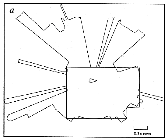
This does not capture the effective error modality seen on a AMR moving through its environment. As the ultrasonic transducer’s angle to the object being ranged varies away from perpendicular, the chances become good that the sound waves will coherently reflect away from the sensor, just as light at a shallow angle reflects off of a mirror. Therefore, the true error behavior of ultrasonic sensors is compound, with a well-understood error distribution near the true value in the case of a successful retro-reflection, and a more poorly-understood set of range values that are grossly larger than the true value in the case of coherent reflection.
Of course the acoustic properties of the material being ranged have direct impact on the sensor’s performance. Again, the impact is discrete, with one material possibly failing to produce a reflection that is sufficiently strong to be sensed by the unit. For example, foam, fur and cloth can, in various circumstances, acoustically absorb the sound waves. A final limitation for ultrasonic ranging relates to bandwidth. Particularly in moderately open spaces, a single ultrasonic sensor has a relatively slow cycle time.
For example, measuring the distance to an object that is 3 m away will take such a sensor 20ms, limiting its operating speed to 50 Hz. But if the robot has a ring of 20 ultrasonic sensors, each firing sequentially and measuring to minimize interference between the sensors, then the ring’s cycle time becomes 0.4s and the overall update frequency of any one sensor is just 2.5 Hz. For a robot conducting moderate speed motion while avoiding obstacles using ultrasonic sensor, this update rate can have a measurable impact on the maximum speed possible while still sensing and avoiding obstacles safely.
Ultrasonic measurements may be limited through barrier layers with large salinity, temperature or vortex differentials.
Laser Rangefinder
The
laser
rangefinder
is
a
ToF
sensor
which
achieves
significant
improvements
over
the
ultrasonic
range
sensor
due
to
the
A mechanical mechanism with a mirror sweeps the light beam to cover the required scene in a plane or even in 3 dimensions, using a rotating mirror. One way to measure the ToF for the light beam is to use a pulsed laser and then measured the elapsed time directly, just as in the ultrasonic solution described in just a little bit. Electronics capable of resolving ps are required in such devices and they are therefore very expensive. A second method is to measure the beat frequency between a frequency modulated continuous wave and its received reflection. Another, even easier method is to measure the phase shift of the reflected light.
Continuous Wave Radar It is a type of radar system where a known stable frequency continuous wave radio energy is transmitted and then received from any reflecting objects. Individual objects can be detected using the Doppler effect, which causes the received signal to have a different frequency from the transmitted signal, allowing it to be detected by filtering out the transmitted frequency.
Doppler-analysis of radar returns can allow the filtering out of slow or non-moving objects, thus offering immunity to interference from large stationary objects and slow-moving clutter. This makes it particularly useful for looking for objects against a background reflector, for instance, allowing a high-flying aircraft to look for aircraft flying at low altitudes against the background of the surface. Because the very strong reflection off the surface can be filtered out, the much smaller reflection from a target can still be seen.
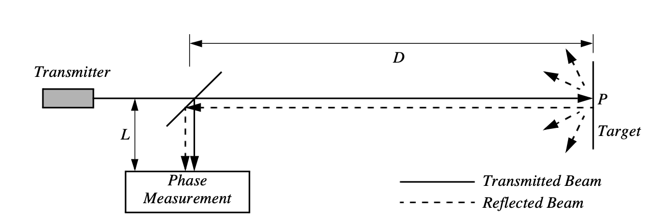
Phase Shift Measurement Near infrared light, which could be from an Light-Emitting Diode (LED) or a laser, is collimated and transmitted from the transmitter in Fig. 2.8 and hits a point in the environment.
For
surfaces
having
a
roughness
greater
than
the
wavelength
of
the
incident
light,
diffuse
reflection
will
occur,
meaning
that
the
light
is
reflected
almost
isotropically
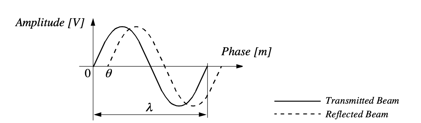
Fig. 2.9 shows how this technique can be used to measure range. The wavelength of the modulating signal obeys the equation where is the speed of light and the modulating frequency.
For example, = 5 MHz , the wavelength is = 60 m .
The total distance covered by the emitted light is:
where and are the distances defined in Fig. 2.8 . The required distance , between the beam splitter and the target, is therefore given by:
where is the electronically measured phase difference between the transmitted and reflected light beams, and the known modulating wavelength. It can be seen that the transmission of a single frequency modulated wave can theoretically result in ambiguous range estimates since
For example if , a target at a range of 5 m would give an indistinguishable phase measurement from a target at 65 m , since each phase angle would be apart.
We therefore define an
As with ultrasonic ranging sensors, an important error mode involves coherent reflection of the energy. With light, this will only occur when striking a highly polishes surface. Practically, a AMR may encounter such surfaces in the form of a polished desktop, file cabinet or of course a mirror. Unlike ultrasonic sensors, laser rangefinders cannot detect the presence of optically transparent materials such as glass, and this can be a significant obstacle in environments, for example museums, where glass is commonly used.
Triangulation-based Active Ranging
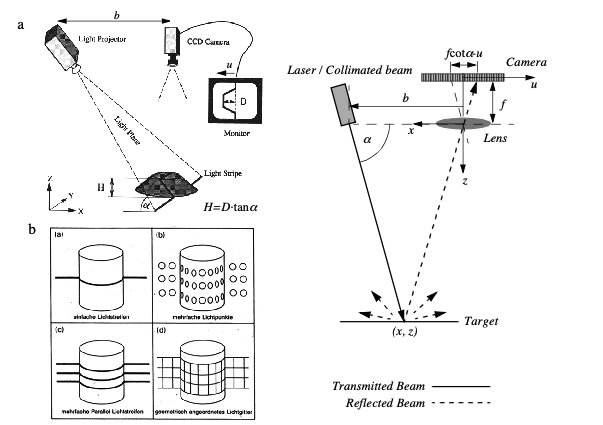
Triangulation-based ranging sensors use geometrical properties in their measuring strategy to establish distance readings to objects. The simplest class of triangulation-based rangers are active because they project a known light pattern (e.g., a point, a line or a texture) onto the environment. The reflection of the known pattern is captured by a receiver and, together with known geometric values, the system can use simple triangulation to establish range measurements. If the receiver measures the position of the reflection along a single axis, we call the sensor an optical triangulation sensor in 1D. If the receiver measures the position of the reflection along two orthogonal axes, we call the sensor a structured light sensor.
Optical Triangulation (1D Sensor)
The principle of optical triangulation in 1D is straightforward, as depicted in Fig. 2.10 .
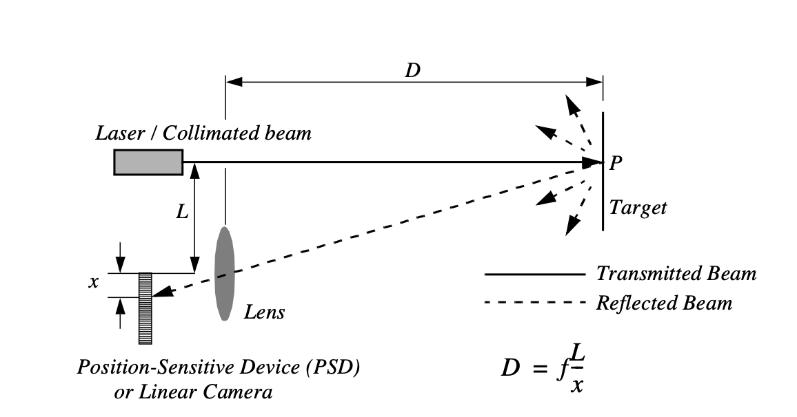
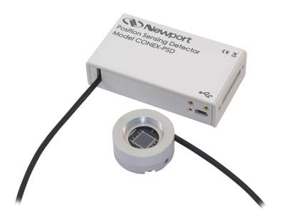
A collimated beam is transmitted toward the target. The reflected light is collected by a lens and projected onto a position sensitive
device
The distance is proportional to
,
therefore the sensor resolution is best for close objects and becomes worse as distance increases. Sensors based on this
principle are used in range sensing up to one or two
m
, but also in high precision industrial measurements with
resolutions far below one
ţ
m
. Optical triangulation devices can provide relatively high accuracy with very good
resolution for close objects. However, the operating range of such a device is normally fairly limited by
It is inexpensive compared to ultrasonic and laser rangefinder sensors.
Although more limited in range than sonar, the optical triangulation sensor has high bandwidth and does not suffer from cross-sensitivities that are more common in the sound domain.
Structured Light (2D Sensor)
If one replaced the linear camera or Position Sensing Device (PSD) of an optical triangulation sensor with a two-dimensional receiver such as a CCD or Complimentary MOS (CMOS) camera, then one can recover distance to a large set of points instead of to only one point. The emitter must project a known pattern, or structured light, onto the environment. Many systems exist which either project light textures, which can be seen in Fig. 2.12 , or emit collimated light by means of a rotating mirror. Yet another popular alternative is to project a laser stripe by turning a laser beam into a plane using a prism. Regardless of how it is created, the projected light has a known structure, and therefore the image taken by the CCD or CMOS receiver can be filtered to identify the pattern’s reflection.
The problem of recovering depth here far simpler than the problem of passive image analysis.
In
passive
image
analysis,
as
we
discuss
later,
existing
features
in
the
environment
must
be
used
to
perform
correlation,
while
the
present
method
projects
a
where is the distance of the lens to the imaging plane. In the limit, the ratio of image resolution to range resolution is defined as the triangulation gain and from equation 4.12 is given by:
This shows that the ranging accuracy, for a given image resolution, is proportional to source/ detector separation and focal length , and decreases with the square of the range . In a scanning ranging system, there is an additional effect on the ranging accuracy, caused by the measurement of the projection angle . From equation 4.12 we see that:
We can summarise the effects of the parameters on the sensor accuracy as follows:
- Baseline Length (b)
-
the smaller is the more compact the sensor can be.The larger is the better the range resolution will be. Note also that although these sensors do not suffer from the correspondence problem, the disparity problem still occurs. As the baseline length b is increased, one introduces the chance that, for close objects, the illuminated point(s) may not be in the receiver’s field of view.
- Detector length and focal length f
-
A larger detector length can provide either a larger field of view or an improved range resolution or partial benefits for both. Increasing the detector length however means a larger sensor head and worse electrical characteristics (increase in random error and reduction of bandwidth). Also, a short focal length gives a large field of view at the expense of accuracy and vice versa.
At one time, laser stripe-based structured light sensors were common on several mobile robot bases as an inexpensive alternative to laser range-finding devices. However, with the in- creasing quality of laser range-finding sensors in the 1990’s the structured light system has become relegated largely to vision research rather than applied mobile robotics.
2.2.2 Motion and Speed Sensors
Some
sensors
directly
measure
the
relative
motion
between
the
robot
and
its
environment.
Since
such
motion
sensors
detect
For
example,
a
pyroelectric
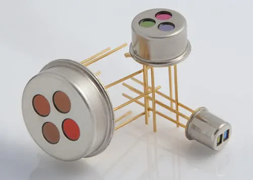
When
someone
walks
across
the
sensor’s
field
of
view,
his
motion
triggers
a
change
in
heat
in
the
sensor’s
reference
frame.
In
the
next
subsection,
we
describe
an
important
type
of
motion
detector
based
on
the
For fast-moving AMR s such as autonomous highway vehicles and unmanned flying vehicles, Doppler-based motion detectors are the obstacle detection sensor of choice.
Doppler Effect
Anyone
who
has
noticed
the
change
in
siren
pitch
when
an
ambulance
approaches
and
then
passes
by
is
familiar
with
the
Doppler
effect.
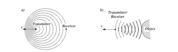
A transmitter emits an electromagnetic or sound wave with a frequency f t. It is either received by a receiver Fig. 2.13 (a) or reflected from an object Fig. 2.13 (b). The measured frequency at the receiver is a function of the relative speed between transmitter and receiver according to
if the transmitter is moving and
if the receiver is moving. In the case of a reflected wave Fig. 2.13 (b) there is a factor of two introduced, since any change x in relative separation affects the round-trip path length by 2 .
In such situations it is generally more convenient to consider the change in frequency , known as the Doppler shift, as opposed to the Doppler frequency notation above.
A current application area is both autonomous and manned highway vehicles. Both micro- wave and laser radar systems have been designed for this environment. Both systems have equivalent range, but laser can suffer when visual signals are deteriorated by environmental conditions such as rain, fog, etc. Commercial microwave radar systems are already avail- able for installation on highway trucks. These systems are called VORAD (vehicle on-board radar) and have a total range of approximately 150m. With an accuracy of approximately 97%, these systems report range rate from 0 to 160 km/hr with a resolution of 1 km/ hr. The beam is approximately 4ř wide and 5ř in elevation. One of the key limitations of radar technology is its bandwidth. Existing systems can provide information on multiple targets at approximately 2 Hz.
2.3 Vision Based Sensors
Vision is our most powerful sense. It provides us with an enormous amount of information about the environment and enables rich, intelligent interaction in dynamic environments. It is therefore not at all surprising that a great deal of effort has been devoted to providing machines with sensors which can at least try to mimic the capabilities of the human vision system.
The
first
step
in
this
process
is
the
creation
of
sensing
devices
that
capture
the
same
raw
information
which
is
the
light
the
human
vision
system
uses.
The
main
topics
which
will
be
described
are
the
two
Of course, these sensors have specific limitations in performance compared to the human eye, and it is important to understand these limitations. Later sections describe vision-based sensors which are commercially available, similar to the sensors discussed previously, along with their disadvantages and most popular applications.
CCD and CMOS Sensors
When
it
comes
to
the
marketplace,
CCD
is
the
most
popular
fundamental
ingredient
for
robotic
vision
systems.
Each
pixel
can
be
thought
of
as
a
In
a
CCD
,
the
reading
process
is
performed
at
one
corner
of
the
CCD
chip.
This requires specialised control circuitry and custom fabrication techniques to ensure the stability of transported charges.
The
photo-diodes
used
in
CCD
chips
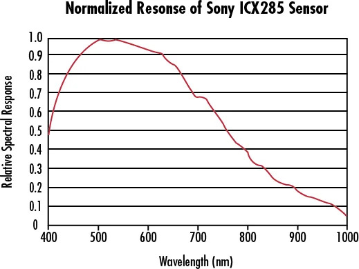
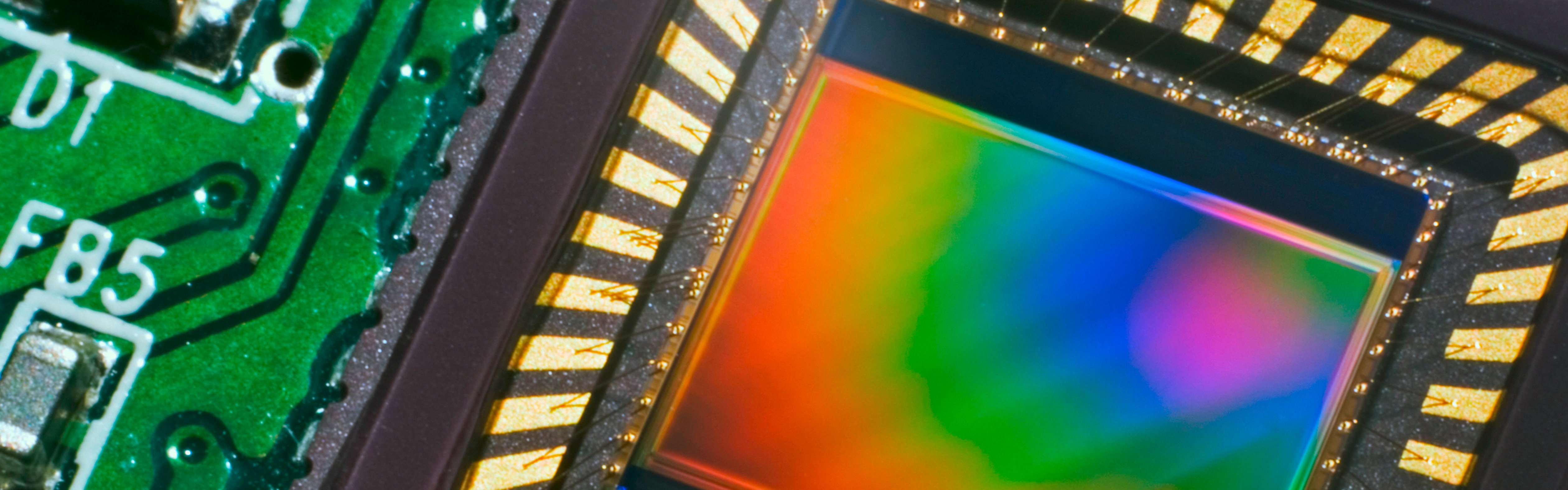
It
is
important
to
remember
that
photodiodes
are
less
sensitive
to
the
ultraviolet
part
of
the
spectrum
and
are
overly
sensitive
to
the
infrared
portion
(e.g.
heat)
which
you
can
see
in
Fig.
2.15
.
You
can
see
that
the
basic
light-measuring
process
is
colourless.
There
are
two


Normally, two
The number of pixels in the system has been effectively cut by a factor of 4, and therefore the image resolution output by the CCD camera will be sacrificed.
The
3-chip
color
camera
avoids
these
problems
by
splitting
the
incoming
light
into
three
Resolution is preserved in this solution, although the 3-chip color cameras are, as one would expect, significantly more expensive and therefore more rarely used in mobile robotics.
Both
3-chip
and
single
chip
color
CCD
cameras
suffer
from
the
fact
that
photo-diodes
are
much
more
sensitive
to
the
near-infrared
end
of
the
spectrum.
This
means
that
the
overall
system
detects
blue
light
much
more
poorly
than
red
and
green.
To
compensate,
the
gain
must
be
increased
on
the
blue
channel,
and
this
introduces
greater
absolute
noise
on
blue
The
CCD
camera
has
several
camera
parameters
that
affect
its
behavior.
In
some
cameras,
these
parameter
values
are
fixed.
In
others,
the
values
are
constantly
changing
based
on
built-in
feedback
loops.
In
higher-end
cameras,
the
user
can
modify
the
values
of
these
parameters
via
software
embedded
into
the
device.
The
iris
position
and
shutter
speed
In
colour
cameras,
an
additional
control
exists
for
white
balance.
Depending
on
the
source
of
illumination
in
a
scene
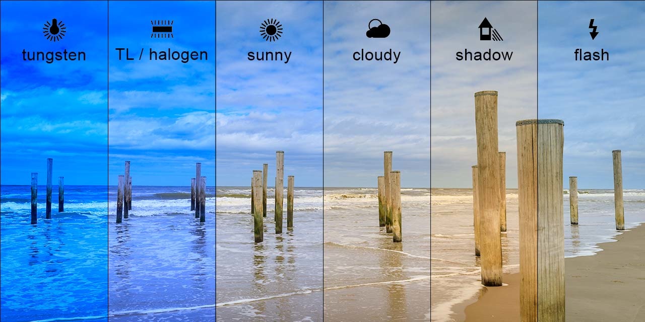
The key disadvantages of CCD cameras are primarily in the areas of inconstancy and dynamic range .
Information : Dynamic Range
Dynamic range in photography describes the ratio between the maximum and minimum measurable light intensities (white and black, respectively). In the real world, one never encounters true white or black - only varying degrees of light source intensity and subject reflectivity. Therefore the concept of dynamic range becomes more complicated, and depends on whether you are describing a capture device (such as a camera or scanner), a display device (such as a print or computer display), or the subject itself.
As mentioned above, a number of parameters can change the brightness and colours with which a camera creates its image.
Manipulating these parameters in a way to provide consistency over time and over environments, for example ensuring a green shirt always looks green, and something dark grey is always dark grey, remains an open problem [41].
The
second
type
of
disadvantages
relates
to
the
behavior
of
a
CCD
chip
in
environments
with
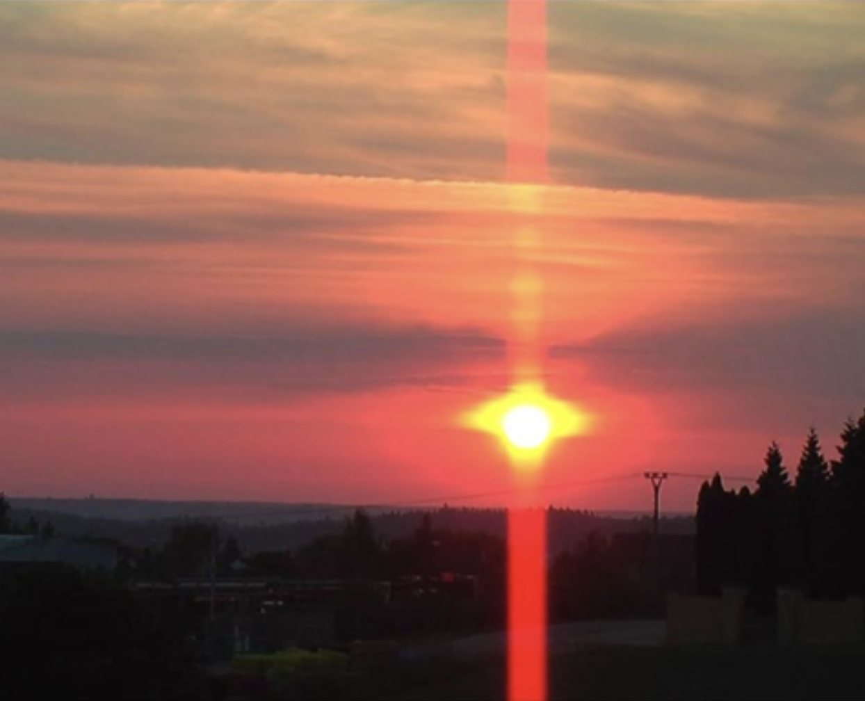
For example, a high quality CCD may have pixels that can hold 40000 electrons. The noise level for reading the well may be 11 electrons, and therefore the dynamic range will be 40,000:11, or 3,600:1, which is 35 dB .
2.3.1 CMOS Technology
The Complementary Metal Oxide Semiconductor (
CMOS
) chip is a significant departure from the
CCD
. Similar to
CCD
, it too
has an array of pixels, but located alongside each pixel are
The pixel-specific circuitry next to every pixel measures and amplifies the pixel’s signal, all in parallel for every pixel in the array.
Using
more
traditional
traces
from
general
semiconductor
chips,
the
resulting
pixel
values
are
all
carried
to
their
destinations.
CMOS
has
a
number
of
advantages
over
CCD
technologies.
First
and
foremost,
there
is
no
need
for
the
specialized
clock
drivers
and
circuitry
required
in
the
CCD
to
transfer
each
pixel’s
clock
down
all
of
the
array
columns
and
across
all
of
its
rows.
This also means that specialized semiconductor manufacturing processes are not required to create CMOS chips.
Therefore, the same production lines that create microchips can create inexpensive CMOS chips as well. The CMOS chip is so much simpler that it consumes significantly less power, it operates with a power consumption a tenth the power consumption of a CCD chip [46].
In a AMR , power is a scarce resource and therefore this is an important advantage.
On the other hand, the CMOS chip also faces several disadvantages.
-
Most importantly, the circuitry next to each pixel consumes valuable real estate on the face of the light-detecting array. Many photons hit the transistors rather than the photodiode, making the CMOS chip significantly less sensitive than an equivalent CCD chip.
-
CMOS , compared to CCD is still finding ground in the marketplace, and as a result, the best resolution that one can purchase in CMOS format continues to be far inferior to the best CCD chips available.
-
CMOS sensors have a lower dynamic range,
-
CMOS sensors have higher levels of noise.
Compared to the human eye, these chips all have worse performance, cross-sensitivity and a limited dynamic range. As a result, vision sensors today continue to be fragile. Only over time, as the underlying performance of imaging chips improves, will significantly more robust vision-based sensors for AMR s be available.
Information : Shot Noise
Shot noise or Poisson noise is a type of noise which can be modeled by a Poisson process.
In electronics shot noise originates from the discrete nature of electric charge. Shot noise also occurs in photon counting in optical devices, where shot noise is associated with the particle nature of light.
2.3.2 Visual Ranging Sensors
Range sensing is extremely important in AMR as it is a basic input for successful obstacle avoidance. As we have seen earlier, a number of sensors are popular in robotics specifically for their ability to recover depth estimates:
ultrasonic, laser rangefinder, optical rangefinder, etc.
It is natural to attempt to implement ranging functionality using vision chips as well. However, a fundamental problem with visual images makes rangefinding relatively difficult.
Any vision chip collapses the three-dimensional world into a two-dimensional image plane, thereby losing depth information. If one can make strong assumptions regarding the size of objects in the world, or their particular colour and reflectance, then one can directly interpret the appearance of the two-dimensional image to recover depth. But such assumptions are rarely possible in real-world AMR applications.
Without such assumptions, a single picture does not provide enough information to recover spatial information.
The
general
solution
is
to
recover
depth
by
looking
at
several
images
of
the
scene
to
gain
more
information,
which
will
be
hopefully
enough
to
at
least
partially
recover
depth.
The
images
used
An alternative is to create different images, not by changing the viewpoint, but by changing the camera geometry, such as the focus position or lens iris. This is the fundamental idea behind depth from focus and depth from defocus techniques. We will now look into the general approach to the depth from focus techniques as it presents a straightforward and efficient way to create a vision-based range sensor.
2.3.3 Depth from Focus
The
depth
from
focus
class
of
techniques
relies
on
the
fact
that
image
properties
not
only
change
as
a
function
of
the
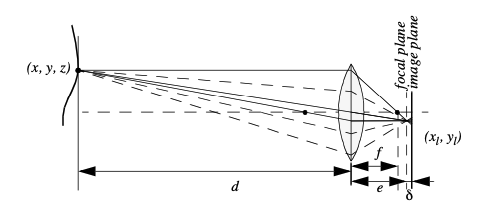
If the image plane is located at distance
from the lens, then for the specific object voxel
where is the diameter of the lens or aperture and is the displacement of the image plan from the focal point.
Given these formulae, several basic optical effects are clear.
For
example,
if
the
aperture
This is consistent with the fact that decreasing the iris aperture opening causes the depth of field to increase until all objects are in focus. Of course, the disadvantage of doing so is that we are allowing less light to form the image on the image plane and so this is practical only in bright circumstances The second property to be deduced from these optics equations relates to the sensitivity of blurring as a function of the distance from the lens to the object.
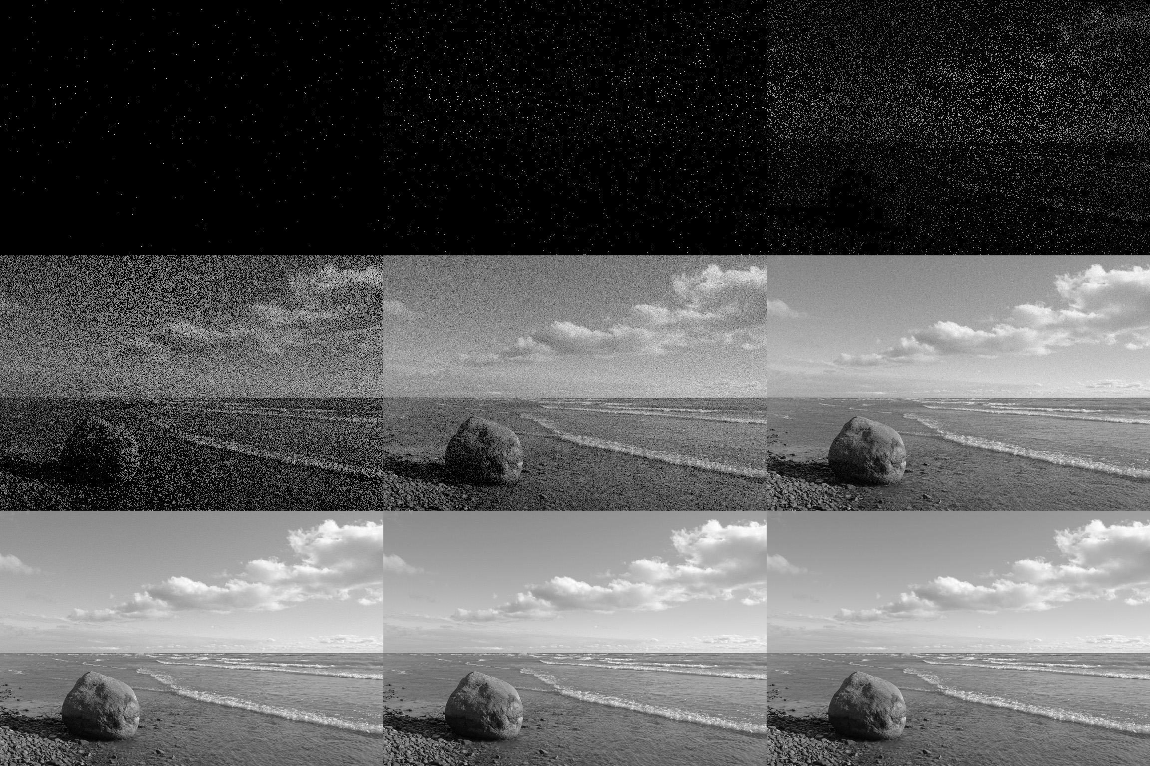
Suppose the image plane is at a fixed distance 1.2 from a lens with diameter L = 0.2 and focal length f = 0.5. We can see from Equation (4.20) that the size of the blur circle R changes proportionally with the image plane displacement . If the object is at distance d = 1, then from Equation (4.19) we can compute e=1 and therefore = 0.2. Increase the object distance to d = 2 and as a result = 0.533. Using Equation (4.20) in each case we can compute R = 0.02 R = 0.08 respectively. This demonstrates high sensitivity for defocusing when the object is close to the lens. In contrast suppose the object is at d = 10. In this case we compute e = 0.526. But if the object is again moved one unit, to d = 11, then we compute e = 0.524. Then resulting blur circles are R = 0.117 and R = 0.129, far less than the quadrupling in R when the obstacle is 1/10 the distance from the lens. This analysis demonstrates the fundamental limitation of depth from focus techniques: they lose sensitivity as objects move further away (given a fixed focal length). Interestingly, this limitation will turn out to apply to virtually all visual ranging techniques, including depth from stereo and depth from motion. Nevertheless, camera optics can be customised for the depth range of the intended application. For example, a "zoom" lens with a very large focal length f will enable range resolution at significant distances, of course at the expense of field of view. Similarly, a large lens diameter, coupled with a very fast shutter speed, will lead to larger, more detectable blur circles. Given the physical effects summarised by the above equations, one can imagine a visual ranging sensor that makes use of multiple images in which camera optics are varied (e.g. image plane displacement ) and the same scene is captured (see Fig. 4.20). In fact this approach is not a new invention. The human visual system uses an abundance of cues and techniques, and one system demonstrated in humans is depth from focus. Humans vary the focal length of their lens continuously at a rate of about 2 Hz. Such approaches, in which the lens optics are actively searched in order to maximise focus, are technically called depth from focus. In contrast, depth from defocus means that depth is recovered using a series of images that have been taken with different camera geometries. Depth from focus methods are one of the simplest visual ranging techniques. To determine the range to an object, the sensor simply moves the image plane (via focusing) until maximizing the sharpness of the object. When the sharpness is maximised, the corresponding position of the image plane directly reports range. Some autofocus cameras and virtually all autofocus video cameras use this technique. Of course, a method is required for measuring the sharpness of an image or an object within the image. The most common techniques are approximate measurements of the sub-image gradient:
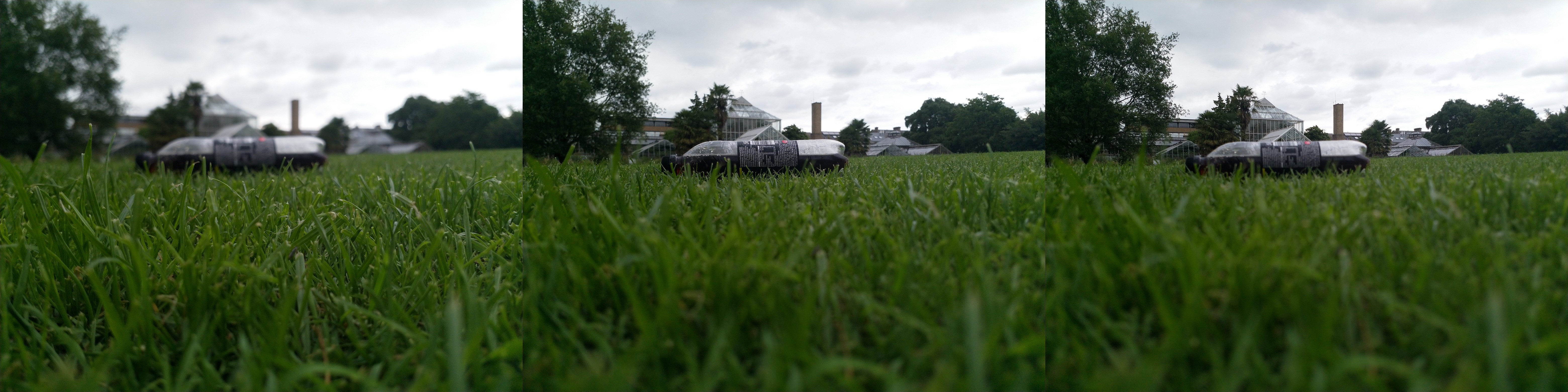
A significant advantage of the horizontal sum of differences technique (Equation (4.21)) is that the calculation can be implemented in analog circuitry using just a rectifier, a low-pass filter and a high-pass filter. This is a common approach in commercial cameras and video recorders. Such systems will be sensitive to contrast along one particular axis, although in practical terms this is rarely an issue. However depth from focus is an active search method and will be slow because it takes time to change the focusing parameters of the camera, using for example a servo-controlled focusing ring. For this reason this method has not been applied to AMR s. A variation of the depth from focus technique has been applied to a AMR , demonstrating obstacle avoidance in a variety of environments as well as avoidance of concave obstacles such as steps and ledges [95]. This robot uses three monochrome cameras placed as close together as possible with different, fixed lens focus positions (Fig. 4.21).
Several times each second, all three frame-synchronised cameras simultaneously capture three images of the same scene. The images are each divided into five columns and three rows, or 15 subregions. The approximate sharpness of each region is computed using a variation of Equation (4.22), leading to a total of 45 sharpness values. Note that Equation 22 calculates sharpness along diagonals but skips one row. This is due to a subtle but important issue. Many cameras produce images in interlaced mode. This means that the odd rows are captured first, then afterwards the even rows are captured. When such a camera is used in dynamic environments, for example on a moving robot, then adjacent rows show the dynamic scene at two different time points, differing by up to 1/30 seconds. The result is an artificial blurring due to motion and not optical defocus. By comparing only even-number rows we avoid this interlacing side effect.
Recall that the three images are each taken with a camera using a different focus position. Based on the focusing position, we call each image close, medium or far. A 5x3 coarse depth map of the scene is constructed quickly by simply comparing the sharpness values of each three corresponding regions. Thus, the depth map assigns only two bits of depth information to each region using the values close, medium and far. The critical step is to adjust the focus positions of all three cameras so that flat ground in front of the obstacle results in medium readings in one row of the depth map. Then, unexpected readings of either close or far will indicate convex and concave obstacles respectively, enabling basic obstacle avoidance in the vicinity of objects on the ground as well as drop-offs into the ground. Although sufficient for obstacle avoidance, the above depth from focus algorithm presents unsatisfyingly coarse range information. The alternative is depth from defocus, the most desirable of the focus-based vision techniques. Depth from defocus methods take as input two or more images of the same scene, taken with different, known camera geometry. Given the images and the camera geometry settings, the goal is to recover the depth information of the three-dimensional scene represented by the images. We begin by deriving the relationship between the actual scene properties (irradiance and depth), camera geometry settings and the image g that is formed at the image plane. The focused image f(x,y) of a scene is defined as follows. Consider a pinhole aperture (L=0) in lieu of the lens. For every point p at position (x,y) on the image plane, draw a line through the pinhole aperture to the corresponding, visible point P in the actual scene. We define f(x,y) as the irradiance (or light intensity) at p due to the light from P. Intuitively, f(x,y) rep- resents the intensity image of the scene perfectly in focus
2.4 Feature Extraction
An
AMR
must be able to
measurements always have error and, therefore, un- certainty associated with them.
Therefore, sensor inputs must be used in a way that enables the robot to interact with its environment successfully in
spite of measurement uncertainty. There are two
The second strategy is to extract information from one or more sensor readings first, gener- ating a higher-level percept that can then be used to inform the robot’s model and perhaps the robot’s actions directly. We call this process feature extraction, and it is this next, op- tional step in the perceptual interpretation pipeline (Fig. 4.34) that we will now discuss.
In practical terms, mobile robots do not necessarily use feature extraction and scene inter- pretation for every activity. Instead, robots will interpret sensors to varying degrees depend- ing on each specific functionality. For example, in order to guarantee emergency stops in the face of immediate obstacles, the robot may make direct use of raw forward-facing range readings to stop its drive motors. For local obstacle avoidance, raw ranging sensor strikes may be combined in an occupancy grid model, enabling smooth avoidance of obstacles meters away. For map-building and precise navigation, the range sensor values and even vision sensor measurements may pass through the complete perceptual pipeline, being sub- jected to feature extraction followed by scene interpretation to minimize the impact of indi- vidual sensor uncertainty on the robustness of the robot’s map-making and navigation skills. The pattern that thus emerges is that, as one moves into more sophisticated, long-term per- ceptual tasks, the feature extraction and scene interpretation aspects of the perceptual pipe- line become essential.
2.4.1 Defining Feature
Features are recognizable structures of elements in the environment. They usually can be extracted from measurements and mathematically described. Good features are always perceivable and easily detectable from the environment. We distinguish between low-level fea- tures (geometric primitives) like lines, circles or polygons and high-level features (objects) such as edges, doors, tables or a trash can. At one extreme, raw sensor data provides a large volume of data, but with low distinctiveness of each individual quantum of data. Making use of raw data has the potential advantage that every bit of information is fully used, and thus there is a high conservation of information. Low level features are abstractions of raw data, and as such provide a lower volume of data while increasing the distinctiveness of each fea- ture. The hope, when one incorporates low level features, is that the features are filtering out poor or useless data, but of course it is also likely that some valid information will be lost as a result of the feature extraction process. High level features provide maximum ab- straction from the raw data, thereby reducing the volume of data as much as possible while providing highly distinctive resulting features. Once again, the abstraction process has the risk of filtering away important information, potentially lowering data utilization.
Although features must have some spatial locality, their geometric extent can range widely. For example, a corner feature inhabits a specific coordinate location in the geometric world. In contract, a visual "fingerprint" identifying a specific room in an office building applies to the entire room, but has a location that is spatially limited to the one, particular room. In mobile robotics, features play an especially important role in the creation of environmen- tal models. They enable more compact and robust descriptions of the environment, helping a mobile robot during both map-building and localization. When designing a mobile robot, a critical decision revolves around choosing the appropriate features for the robot to use. A number of factors are essential to this decision:
- Target Environment
-
For geometric features to be useful, the target geometries must be readily detected in the actual environment. For example, line features are extremely useful in office building environments due to the abundance of straight walls segments while the same feature is virtually useless when navigating Mars.
- Available Sensors
-
Obviously the specific sensors and sensor uncertainty of the robot im- pacts the appropriateness of various features. Armed with a laser rangefinder, a robot is well qualified to use geometrically detailed features such as corner features due to the high qual- ity angular and depth resolution of the laser scanner. In contrast, a sonar-equipped robot may not have the appropriate tools for corner feature extraction.
- Computational Power
-
Vision-based feature extraction can effect a significant computa- tional cost, particularly in robots where the vision sensor processing is performed by one of the robot’s main processors.
- Environment representation
-
Feature extraction is an important step toward scene inter- pretation, and by this token the features extracted must provide information that is consonant with the representation used for the environment model. For example, non-geometric vi- sion-based features are of little value in purely geometric environment models but can be of great value in topological models of the environment. Figure 4.35 shows the application of two different representations to the task of modeling an office building hallway. Each ap- proach has advantages and disadvantages, but extraction of line and corner features has much more relevance to the representation on the left. Refer to Chapter 5, Section 5.5 for a close look at map representations and their relative tradeoffs. In the following two sections, we present specific feature extraction techniques based on the two most popular sensing modalitites of mobile robotics: range sensing and visual appear- ance-based sensing.
2.4.2 Using Range Data
Most of today’s features extracted from ranging sensors are geometric primitives such as line segments or circles. The main reason for this is that for most other geometric primitives the parametric description of the features becomes too complex and no closed form solution exists. Here we will describe line extraction in detail, demonstrating how the uncertainty models presented above can be applied to the problem of combining multiple sensor mea- surements. Afterwards, we briefly present another very successful feature for indoor mobile robots, the corner feature, and demonstrate how these features can be combined in a single representation.
Line Extraction
Geometric feature extraction is usually the process of comparing and matching measured sensor data against a predefined description, or template, of the expect feature. Usually, the system is overdetermined in that the number of sensor measurements exceeds the number of feature parameters to be estimated. Since the sensor measurements all have some error, there is no perfectly consistent solution and, instead, the problem is one of optimization. One can, for example, extract the feature that minimizes the discrepancy with all sensor measurements used (e.g. least squares estimation). In this section we present an optimization-based solution to the problem of extracting a line feature from a set of uncertain sensor measurements. For greater detail than is presented be- low, refer to [19], pp. 15 and 221.
Probabilistic Line Extraction
4.36. There is uncertainty associated with each of the noisy range sensor measurements, and so there is no single line that passes through the set. Instead, we wish to select the best pos- sible match, given some optimization criterion. More formally, suppose n ranging measurement points in polar coordinates x = ( , ) iii are produced by the robot’s sensors. We know that there is uncertainty associated with each measurement, and so we can model each measurement using two random variables X = ( P , Q ) . In this analysis we assume that uncertainty with respect to the actual value iii of P and Q are independent. Based on Equation (4.56) we can state this formally: Furthermore, we will assume that each random variable is subject to a Gaussian probability density curve, with a mean at the true value and with some specified variance: Given some measurement point (, ) , we can calculate the corresponding Euclidean co- ordinatesasx = cos andy = sin. Iftherewerenoerror,wewouldwanttofinda line for which all measurements lie on that line: Of course there is measurement error, and so this quantity will not be zero. When it is non- zero, this is a measure of the error between the measurement point (, ) and the line, spe- cifically in terms of the minimum orthogonal distance between the point and the line. It is always important to understand how the error that shall be minimized is being measured. For example a number of line extraction techniques do not minimize this orthogonal point- line distance, but instead the distance parallel to the y-axis between the point and the line. A good illustration of the variety of optimization criteria is available in [18] where several algorithms for fitting circles and ellipses are presented which minimize algebraic and geo- metric distances. For each specific ( , ) , we can write the orthogonal distance d between ( , ) and iiiii the line as: