7

Computer Vision using Convolutional Neural Networks

7.1 Introduction

It wasn’t until recently computers were able to reliably perform seemingly easy tasks such as detecting a cat ^{1 1} As it is known, internet was invented for sharing cat pictures, therefore their detection is paramount. in a picture or recognising spoken words. Why are these tasks so effortless to us humans? The answer lies in the fact that perception largely takes place outside the realm of our control , within specialized visual, auditory, and other sensory modules in our brains. By the time sensory information reaches our consciousness, it is already imbued with high-level features . For example:

Therefore, we cannot trust our subjective experience.

Perception is NOT a trivial task, and to understand it we must look at how our sensory modules work. CNN s emerged from the study of the brain’s visual cortex, and they have been used in computer image recognition since the 1980s [57]. Over the last 10 years, thanks to the increase in computational power, the amount of available training data, and a much better methods developed for training deep nets, CNN s have managed to achieve impressive performance on some complex visual tasks. Some examples of their application include:

• Search services: Such as connecting users in the web to the software they need to find [58], [59],

• Self-driving cars: Such as detecting the colours on a traffic light [60], or detecting the road lines during driving [61],

• Automatic video classification : i.e., detecting videos and categorising based on content [62],

• Object Detection: Such as detecting objects in an image [20].

In addition, CNN s are not restricted to visual perception:

However, as our topic is Image Processing , we will focus on its visual applications. In this chapter we will explore where CNN s came from, what their building blocks look like, and how to implement them using tf.keras. Then we will discuss some of the best CNN architectures, as well as other visual tasks, including object detection ^{2 2} classifying multiple objects in an image and placing bounding boxes around them and semantic segmentation..

7.2 Visual Cortex Architecture

David H. Hubel and Torsten Wiesel performed a series of experiments on cats in 1958 and 1959 (and a few years later on monkeys), giving crucial insights into the structure of the visual cortex ^{3 3} the authors received the Nobel Prize in Physiology or Medicine in 1981 for their work [63]. What is important to us is, they showed that many neurons in the visual cortex have a small local receptive field , meaning they react only to visual stimuli located in a limited region of the visual field . A diagram showcasing this phenomenon can be seen in Fig. 7.2 , in which the local receptive fields of five neurons are represented by dashed circles. The receptive fields of different neurons may overlap, and together they tile the whole visual field.

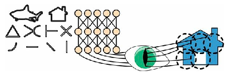
In addition to the previous revelation of how neurons work, they showed some neurons react ONLY to images of horizontal lines, while others react ONLY to lines with different orientations ^{4 4} two neurons may have the same receptive field but react to different line orientations . They also noticed that some neurons have larger receptive fields, and they react to more complex patterns that are combinations of the lower-level patterns. These observations led to the idea that the higher-level neurons are based on the outputs of neighboring lower-level neurons. (in Fig. 7.2 , observe that each neuron is connected only to nearby neurons from the previous layer). This powerful architecture is able to detect all sorts of complex patterns in any area of the visual field. These studies of the visual cortex inspired the neocognitron [64], introduced in 1980, which gradually evolved into what we now call CNN . An important milestone was a 1998 paper by Yann LeCun et.al. which introduced the famous LeNet-5 architecture, which became widely used by banks to recognize handwritten digits on checks [65]. This architecture has some building blocks were are familiar with:

• Fully connected layers,

• Sigmoid activation functions ^{5 5} A function allowing non-linear properties for the neural network. ,

but it also introduces two new building blocks:

• convolutional layers

• pooling layers.

Which will, of course, will be our focus of attention this chapter.

7.3 Convolutional Layers

The most important building block of a CNN is the convolutional layer :

The neurons are only connected to pixels in their receptive fields which its graphical representation can be seen in Fig. 7.3 .

In turn, each neuron in the second convolutional layer is connected only to neurons located within a small rectangle in the first layer. This architecture allows the network to concentrate on small low-level features in the first hidden layer, then assemble them into larger higher-level features in the next hidden layer, and so on. This hierarchical structure is common in real-world images, which is one of the reasons why CNN s work so well for image recognition. A neuron located in row $i$ , column $j$ of a given layer is connected to the outputs of the neurons in the previous layer located in rows $i$ to $i+f_h^{}-1$ , columns $j$ to $j+f_w^{}-1$ , where $f_h^{}$ and $f_w^{}$ are the height and width of the receptive field which can be observed in Fig. ??.

It is also possible to connect a large input layer to a much smaller layer by spacing out the receptive fields, shown in Fig. ??.

This significantly decreases the model’s computational complexity. The horizontal or vertical step size from one receptive field to the next is called the stride . In Fig. ??, a 5-by-7 input layer (plus zero padding) is connected to a 3-by-4 layer, using 3-by-3 receptive fields and a stride of 2 ^{7 7} in this example the stride is the same in both directions, but it does not have to be so . A neuron located in row $i$ , column $j$ in the upper layer is connected to the outputs of the neurons in the previous layer located in rows iŒsh toiŒsh +fh -1,columnsjŒsw to j Œ sw + fw - 1, where sh and sw are the vertical and horizontal strides.

7.3.1 Filters

A neuron’s weights can be represented as a small image the size of the receptive field. For example, Fig. 7.5 shows two (2) possible sets of weights, called filters ^{8 8} The terms convolution kernels, or kernels are also used .

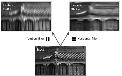
The first one is represented as a black square with a vertical white line in the middle.

Neurons using these weights will ignore everything in their receptive field except for the central vertical line ^{9 9} since all inputs will be multiplied by 0, except for the ones in the central vertical line . The second filter is a black square with a horizontal white line in the middle. Neurons using these weights will ignore everything in their receptive field except for the central horizontal line. If all neurons in a layer use the same vertical line filter (and the same bias term), and we feed the network the input image shown in Fig. 7.5 (the bottom image), the layer will output the top-left image. Notice that the vertical white lines get enhanced while the rest gets blurred. Similarly, the upper-right image is what we get if all neurons use the same horizontal line filter. Notice the horizontal white lines get enhanced while the rest is blurred out. Therefore, a layer full of neurons using the same filter outputs a feature map , which highlights the areas in an image that activate the filter the most.

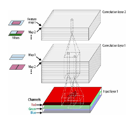
7.3.2 Stacking Multiple Feature Maps

Up to now, for simplicity, We represented the output of each convolutional layer as a 2D layer, but in reality a convolutional layer has multiple filters ^{10 10} The number of filters is left up to the programmer and outputs one feature map per filter, so it is more accurately represented in 3D, which can be seen in Fig. 7.6 . It has one neuron per pixel in each feature map, and all neurons within a given feature map share the same parameters (i.e., the same kernel and bias term). Neurons in different feature maps use different parameters. A neuron’s receptive field is the same as described earlier, but it extends across all the feature maps of the previous layer. In short, a convolutional layer simultaneously applies multiple trainable filters to its inputs, making it capable of detecting multiple features anywhere in its inputs.

Input images are also composed of multiple sublayers: one per color channel. As we already now, there are typically three: red, green, and blue (RGB). Grayscale images have just one channel, but some images may have many more-for example, satellite images that capture extra light frequencies

Specifically, a neuron located in row $i$ , column $j$ of the feature map $k$ in a given convolutional layer $l$ is connected to the outputs of the neurons in the previous layer $l-1$ , located in rows $i\times s_h^{}$ to $i\times s_h^{}+f_h^{}-1$ and columns $j\times s_w^{}$ to $j\times s_w^{}+f_w^{}-1$ ,across all feature maps( in layer $l-1$ ).

This definition can be summarised in one big mathematical equation: it shows how to compute the output of a given neuron in a convolutional layer.

Let’s try to understand the variables:

• $z_{i,j,k}^{}$ is the output of the neuron located in row $i$ , column $j$ in feature map $k$ of the convolutional layer (layer $l$ ).

• $s_h^{},s_w^{}$ are the vertical and horizontal strides, $f_h^{},f_w^{}$ are the height and width of the receptive field, and $f_n^{\prime }$ is the number of feature maps in the previous layer ( $l-1$ ).

• $x_{i_{}^{\prime },j_{}^{\prime },k_{}^{\prime }}^{}$ is the output of the neuron located in layer $l-1$ , row $i_{}^{\prime }$ , column $j_{}^{\prime }$ , feature map $k_{}^{\prime }$ , or channel $k_{}^{\prime }$ if the previous layer is the input layer.

• $\underset{¯}{[}k]$ is the bias term for feature map $k$ (in layer $l$ ). Think of it as a knob that tweaks the overall brightness of the feature map $k$ .

• $w_{u,v,k_{}^{\prime },k_{}^{}}^{}$ is the connection weight between any neuron in feature map $k$ of the layer $l$ and its input located at row $u$ , column $v$ (relative to the neuron’s receptive field), and feature map $k_{}^{\prime }$ .

7.3.3 Implementing Convolutional Layers with Keras

As with every ML application, we load and preprocess a couple of sample images, using sklearn ’s load_sample_image() function and Keras’s CenterCrop and Rescaling layers:

from sklearn.datasets import load_sample_images 
import tensorflow as tf 
 
images = load_sample_images()["images"] 
images = tf.keras.layers.CenterCrop(height=70, width=120)(images) 
images = tf.keras.layers.Rescaling(scale=1 / 255)(images)

Let’s look at the shape of the images tensor ^{11 11} A tensor is a generalization of vectors and matrices to potentially higher dimensions. :

print(images.shape)

(2, 70, 120, 3)

It’s a 4D tensor. Let’s see why this is a 4D matrix. There are two (2) sample images, which explains the first dimension. Then each image is 70 -by- 120 , as that’s the size we specified when creating the CenterCrop layer ^{12 12} the original images were 427-by-640 . This explains the second and third dimensions. And lastly, each pixel holds one value per colour channel, and there are three (3) of them:

Now let’s create a 2D convolutional layer and feed it these images to see what comes out. For this, Keras provides a Convolution2D layer, alias Conv2D. Under the hood, this layer relies on TensorFlow’s tf.nn.conv2d() operation.

Let’s create a convolutional layer with 32 filters, each of size 7-by-7 (using kernel_size=7, which is equivalent to using kernel_size=(7 , 7) ), and apply this layer to our small batch of two (2) images:

tf.random.set_seed(42)  # extra code  ensures reproducibility 
conv_layer = tf.keras.layers.Conv2D(filters=32, kernel_size=7) 
fmaps = conv_layer(images)

Now let’s look at the output’s shape:

print(fmaps.shape)

(2, 64, 114, 32)

The output shape is similar to the input shape, with two (2) main differences.

1.

There are 32 channels instead of 3. This is because we set filters=32, so we get 32 output feature maps: instead of the intensity of red, green, and blue at each location, we now have the intensity of each feature at each location.

2.

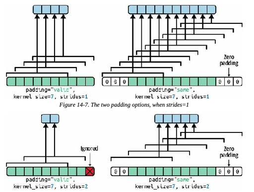
The height and width have both shrunk by 6 pixels. This is due to the fact that the Conv2D layer does NOT use any zero-padding by default, which means that we lose a few pixels on the sides of the output feature maps, depending on the size of the filters. In this case, since the kernel size is 7, we lose 6 pixels horizontally and 6 pixels vertically (i.e., 3 pixels on each side).

If instead we set padding="same", then the inputs are padded with enough zeros on all sides to ensure that the output feature maps end up with the same size as the inputs (hence the name of this option):

These two padding options are illustrated in Fig. 7.8 . For simplicity, only the horizontal dimension is shown here, but of course the same logic applies to the vertical dimension as well.

If the stride is greater than 1 (in any direction), then the output size will not be equal to the input size, even if padding="same". For example, if we set strides=2 (or equivalently strides=(2, 2) ), then the output feature maps will be 35-by-60: halved both vertically and horizontally.

Fig. 7.8 shows what happens when strides=2 , with both padding options.

If we are curious, this is how the output size is computed:

• With padding="valid", if the width of the input is ih, then the output width is equal to (ih - fh + sh) / sh, rounded down. Recall that fh is the kernel width, and sh is the horizontal stride. Any remainder in the division corresponds to ignored columns on the right side of the input image. The same logic can be used to compute the output height, and any ignored rows at the bottom of the image.

• With padding="same", the output width is equal to ih / sh, rounded up. To make this possible, the appropriate number of zero columns are padded to the left and right of the input image (an equal number if possible, or just one more on the right side). Assuming the output width is ow, then the number of padded zero columns is (ow - 1) Œ sh + fh - ih. Again, the same logic can be used to compute the output height and the number of padded rows.

Now let’s look at the layer’s weights (which were noted wu, v, k’, k and bk in Equation 14-1). Just like a Dense layer, a Conv2D layer holds all the layer’s weights, including the kernels and biases. The kernels are initialized randomly, while the biases are initialized to zero. These weights are accessible as TF variables via the weights attribute, or as NumPy arrays via the get_weights() method:

The kernels array is 4D, and its shape is [ kernel_height, kernel_width, input_channels, output_channels ]. The biases array is 1D, with shape [ output_channels ]. The number of output channels is equal to the number of output feature maps, which is also equal to the number of filters. Most importantly, note that the height and width of the input images do not appear in the kernel’s shape: this is because all the neurons in the output feature maps share the same weights, as explained earlier. This means that we can feed images of any size to this layer, as long as they are at least as large as the kernels, and if they have the right number of channels (three in this case).

Lastly, we will generally want to specify an activation function (such as ReLU) when creating a Conv2D layer, and also specify the corresponding kernel initializer. This is for the same reason as for Dense layers: a convolutional layer performs a linear operation, so if we stacked multiple convolutional layers without any activation functions they would all be equivalent to a single convolutional layer, and they wouldn’t be able to learn anything really complex.

As we can see, convolutional layers have quite a few hyperparameters: filters, kernel_size, padding, strides, activation, kernel_initializer, etc. As always, we can use cross-validation to find the right hyperparameter values, but this is very time-consuming. We will discuss common CNN architectures later in this chapter, to give you some idea of which hyperparameter values work best in practice.

7.3.4 Memory Requirements

Another challenge with CNN s is that the convolutional layers require a huge amount of RAM. This is especially true during training, because the reverse pass of back-propagation requires all the intermediate values computed during the forward pass.

As an example, consider a convolutional layer with 200 5-by-5 filters, with stride 1 and "same" padding. If the input is a 150-by-100 RGB image, then the number of parameters is (5-by-5-by-3+1) Œ 200 = 15,200 ^{13 13} the + 1 corresponds to the bias terms , which is fairly small compared to a fully connected layer. However, each of the 200 feature maps contains 150 Œ 100 neurons, and each of these neurons needs to compute a weighted sum of its 5-by-5-by-3 = 75 inputs: that’s a total of 225 million float multiplications.

Not as bad as a fully connected layer, but still quite computationally intensive. Moreover, if the feature maps are represented using 32-bit floats, then the convolutional layer’s output will occupy $200\times 150\times 100\times 32$ = 96 million bits (12 MB) of RAM. 8 And that’s just for one instance-if a training batch contains 100 instances, then this layer will use up 1.2 GB of RAM.

During inference (i.e., when making a prediction for a new instance) the RAM occupied by one layer can be released as soon as the next layer has been computed, so we only need as much RAM as required by two consecutive layers. But during training everything computed during the forward pass needs to be preserved for the reverse pass, so the amount of RAM needed is (at least) the total amount of RAM required by all layers.

Now let’s look at the second common building block of CNN s: the pooling layer .

7.4 Pooling Layer

The goal of a pooling layer is to subsample (i.e., shrink) the input image to reduce the computational load, the memory usage, and the number of parameters ^{14 14} This limits the risk of overfitting .

Just like in convolutional layers, each neuron in a pooling layer is connected to the outputs of a limited number of neurons in the previous layer, located within a small rectangular receptive field . We must define its size, the stride, and the padding type, just like before.

However, a pooling neuron has NO weights. All it does is aggregate the inputs using an aggregation function such as the max or mean.

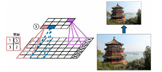
Fig. 7.9 shows a max pooling layer , which is the most common type of pooling layer. In this example, we use a 2-by-2 pooling kernel, with a stride of 2 and no padding. Only the max input value in each receptive field makes it to the next layer, while the other inputs are dropped. For example, in the lower-left receptive field in Fig. 7.9 , the input values are 1, 5, 3, 2, so only the max value, 5, is propagated to the next layer. Because of the stride of 2, the output image has half the height and half the width of the input image (rounded down since we use no padding).

Other than reducing computations, memory usage, and the number of parameters, a max pooling layer also introduces some level of invariance ^{15 15} In the context of computer vision, it means that we can recognize an object as an object, even when its appearance varies in some way. to small translations, as shown in Fig. 7.10 .

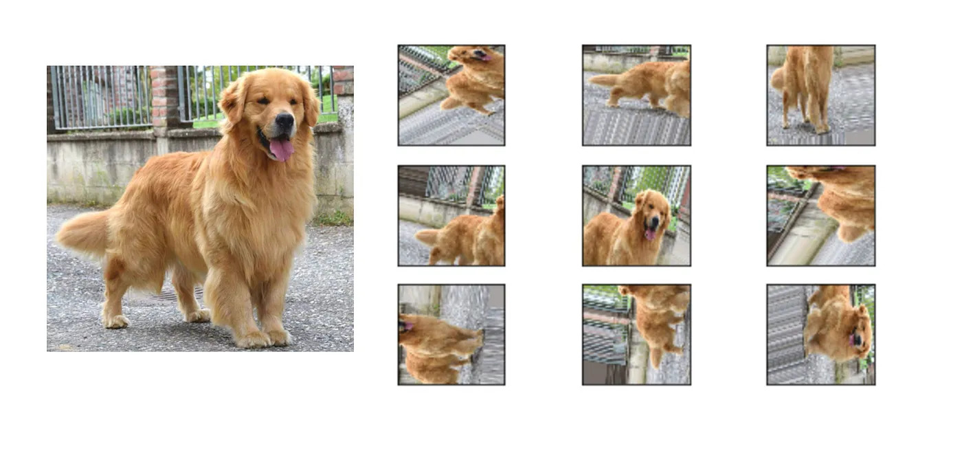
Here we assume that the bright pixels have a lower value than dark pixels, and we consider three images (A, B, C) going through a max pooling layer with a 2-by-2 kernel and stride 2. Images B and C are the same as image A, but shifted by one and two pixels to the right. As we can see, the outputs of the max pooling layer for images A and B are identical. This is what translation invariance means. For image C, the output is different: it is shifted one pixel to the right (but there is still 50% invariance). By inserting a max pooling layer every few layers in a CNN , it is possible to get some level of translation invariance at a larger scale.

However, max pooling has some downsides too. It’s obviously very destructive: even with a tiny 2 Œ 2 kernel and a stride of 2, the output will be two times smaller in both directions (so its area will be four times smaller), simply dropping 75% of the input values. And in some applications, invariance is not desirable. Take semantic segmentation ^{16 16} The task of classifying each pixel in an image according to the object that pixel belongs to .

For this case, if the input image is translated by one pixel to the right, the output should also be translated by one pixel to the right. The goal in this case is equivariance, not invariance: a small change to the inputs should lead to a coresponding small change in the output.

7.5 Implementing Pooling Layers with Keras

The following code creates a MaxPooling2D layer, alias MaxPool2D , using a 2-by-2 kernel. The strides default to the kernel size, so this layer uses a stride of 2 (horizontally and vertically). By default, it uses "valid" padding (i.e., no padding at all):

max_pool = tf.keras.layers.MaxPool2D(pool_size=2)

To create an average pooling layer, just use AveragePooling2D, alias AvgPool2D , instead of MaxPool2D. As we might expect, it works exactly like a max pooling layer, except it computes the mean rather than the max. Average pooling layers used to be very popular, but people mostly use max pooling layers now, as they generally perform better. This may seem surprising, since computing the mean generally loses less information than computing the max. But on the other hand, max pooling preserves only the strongest features, getting rid of all the meaningless ones, so the next layers get a cleaner signal to work with. Moreover, max pooling offers stronger translation invariance than average pooling, and it requires slightly less compute.

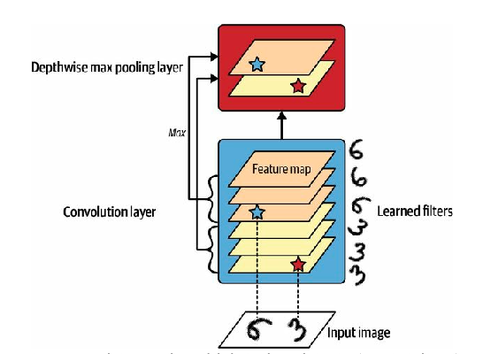
Note that max pooling and average pooling can be performed along the depth dimension instead of the spatial dimensions, although it’s not as common. This can allow the CNN to learn to be invariant to various features. For example, it could learn multiple filters, each detecting a different rotation of the same pattern (such as handwritten digits seen in Fig. 7.11 ), and the depthwise max pooling layer would ensure that the output is the same regardless of the rotation. The CNN could similarly learn to be invariant to anything: thickness, brightness, skew, color, and so on.

Keras does not include a depthwise max pooling layer, but it’s not too difficult to implement a custom layer for that:

class DepthPool(tf.keras.layers.Layer): 
   def __init__(self, pool_size=2, **kwargs): 
      super().__init__(**kwargs) 
      self.pool_size = pool_size 
 
   def call(self, inputs): 
      shape = tf.shape(inputs)  # shape[-1] is the number of channels 
      groups = shape[-1] // self.pool_size  # number of channel groups 
      new_shape = tf.concat([shape[:-1], [groups, self.pool_size]], axis=0) 
      return tf.reduce_max(tf.reshape(inputs, new_shape), axis=-1)

This layer reshapes its inputs to split the channels into groups of the desired size (pool_size), then it uses tf.reduce_max() to compute the max of each group. This implementation assumes that the stride is equal to the pool size, which is generally what we want. Alternatively, we could use TensorFlow’s tf.nn.max_pool() operation, and wrap in a Lambda layer to use it inside a Keras model, but sadly this op does not implement depthwise pooling for the GPU, only for the CPU.

One last type of pooling layer that we will often see in modern architectures is the global average pooling layer. It works very differently: all it does is compute the mean of each entire feature map (it’s like an average pooling layer using a pooling kernel with the same spatial dimensions as the inputs). This means that it just outputs a single number per feature map and per instance. Although this is of course extremely destructive (most of the information in the feature map is lost), it can be useful just before the output layer, as we will see later in this chapter. To create such a layer, simply use the GlobalAveragePooling2D class, alias GlobalAvgPool2D:

7.6 CNN Architectures

Typical CNN architectures stack a few convolutional layers (each one generally followed by a ReLU layer), then a pooling layer, then another few convolutional layers (+ReLU), then another pooling layer, and so on. The image gets smaller and smaller as it progresses through the network, but it also typically gets deeper and deeper (i.e., with more feature maps), thanks to the convolutional layers (see Fig. ??). At the top of the stack, a regular feedforward neural network is added, composed of a few fully connected layers (+ReLUs), and the final layer outputs the prediction (e.g., a softmax layer that outputs estimated class probabilities).

Here is how we can implement a basic CNN to tackle the Fashion MNIST dataset.

Let’s first download and allocated the traning/testing.

import numpy as np 
 
mnist = tf.keras.datasets.fashion_mnist.load_data() 
(X_train_full, y_train_full), (X_test, y_test) = mnist 
X_train_full = np.expand_dims(X_train_full, axis=-1).astype(np.float32) / 255 
X_test = np.expand_dims(X_test.astype(np.float32), axis=-1) / 255 
X_train, X_valid = X_train_full[:-5000], X_train_full[-5000:] 
y_train, y_valid = y_train_full[:-5000], y_train_full[-5000:]

from functools import partial 
 
tf.random.set_seed(42)  # extra code  ensures reproducibility 
DefaultConv2D = partial(tf.keras.layers.Conv2D, kernel_size=3, padding="same", 
                 activation="relu", kernel_initializer="he_normal") 
model = tf.keras.Sequential([ 
   DefaultConv2D(filters=64, kernel_size=7, input_shape=[28, 28, 1]), 
   tf.keras.layers.MaxPool2D(), 
   DefaultConv2D(filters=128), 
   DefaultConv2D(filters=128), 
   tf.keras.layers.MaxPool2D(), 
   DefaultConv2D(filters=256), 
   DefaultConv2D(filters=256), 
   tf.keras.layers.MaxPool2D(), 
   tf.keras.layers.Flatten(), 
   tf.keras.layers.Dense(units=128, activation="relu", 
                  kernel_initializer="he_normal"), 
   tf.keras.layers.Dropout(0.5), 
   tf.keras.layers.Dense(units=64, activation="relu", 
                  kernel_initializer="he_normal"), 
   tf.keras.layers.Dropout(0.5), 
   tf.keras.layers.Dense(units=10, activation="softmax") 
])

Let’s go through this code:

1.

We use the functools.partial() function to define DefaultConv2D, which acts just like Conv2D but with different default arguments: a small kernel size of 3, "same" padding, the ReLU activation function, and its corresponding He initializer .

2.

We create the Sequential model. Its first layer is a DefaultConv2D with 64 fairly large filters (7-by-7). It uses the default stride of 1 because the input images are not very large. It also sets input_shape=[28, 28, 1], as the images are 28-by-28 pixels, with a single color channel (i.e., grayscale).

3.

When we load the Fashion MNIST dataset, we need to make sure each image has this shape. Therefore we may require to use np.reshape() or np.expanddims() to add the channels dimension or we could use a Reshape layer as the first layer in the model.

4.

We then add a max pooling layer that uses the default pool size of 2, so it divides each spatial dimension by a factor of 2.

5.

We repeat the same structure twice: two convolutional layers followed by a max pooling layer. For larger images, we could repeat this structure several more times. The number of repetitions is a hyperparameter we can tune

Observe the number of filters doubles as we climb up the CNN toward the output layer (it is initially 64, then 128, then 256): it makes sense for it to grow, since the number of low-level features is often fairly low (e.g., small circles, horizontal lines), but there are many different ways to combine them into higher-level features. It is a common practice to double the number of filters after each pooling layer: since a pooling layer divides each spatial dimension by a factor of 2, we can afford to double the number of feature maps in the next layer without fear of exploding the number of parameters, memory usage, or computational load.

6.

Next is the fully connected network, composed of two hidden dense layers and a dense output layer. Since it’s a classification task with 10 classes, the output layer has 10 units, and it uses the softmax activation function. Note that we must flatten the inputs just before the first dense layer, since it expects a 1D array of features for each instance. We also add two dropout layers, with a dropout rate of 50% each, to reduce overfitting.

If we compile this model using the "sparse_categorical_crossentropy" loss and we fit the model to the Fashion MNIST training set, it should reach over 92% accuracy on the test set.

model.compile(loss="sparse_categorical_crossentropy", optimizer="nadam", 
          metrics=["accuracy"]) 
history = model.fit(X_train, y_train, epochs=10, 
              validation_data=(X_valid, y_valid)) 
score = model.evaluate(X_test, y_test) 
X_new = X_test[:10]  # pretend we have new images 
y_pred = model.predict(X_new)

Over the years, variants of this fundamental architecture have been developed, leading to amazing advances in the field. A good measure of this progress is the error rate in competitions such as the ILSVRC ImageNet challenge. In this competition, the top-five error rate for image classification -that is, the number of test images for which the system’s top five predictions did not include the correct answer-fell from over 26% to less than 2.3% in just six years. The images are fairly large (e.g., 256 pixels high) and there are 1,000 classes, some of which are really subtle (try distinguishing 120 dog breeds).

Looking at the evolution of the winning entries is a good way to understand how CNN s work, and how research in deep learning progresses. We will first look at:

• LeNet-5 architecture (1998)

• AlexNet (2012),

• GoogLeNet (2014),

• ResNet (2015),

• SENet (2017).

In addition, we will also briefly look at more architectures, including Xception, ResNeXt, DenseNet, MobileNet, CSPNet, and EfficientNet.

7.6.1 LeNet-5

The LeNet-5 architecture is perhaps the most widely known CNN architecture. As mentioned, it was created by Yann LeCun in 1998 and has been widely used for handwritten digit recognition (MNIST).

As we can see, this looks pretty similar to our Fashion MNIST model: a stack of convolutional layers and pooling layers, followed by a dense network. Perhaps the main difference with more modern classification CNN s is the activation functions: today, we would use ReLU instead of tanh and softmax instead of RBF.

7.6.2 AlexNet

The AlexNet CNN architecture won the 2012 ILSVRC challenge by a large margin: it achieved a top-five error rate of 17%, while the second best competitor achieved only 26%! AlexaNet was developed by Alex Krizhevsky, Ilya Sutskever, and Geoffrey Hinton. It is similar to LeNet-5, only much larger and deeper, and it was the first to stack convolutional layers directly on top of one another, instead of stacking a pooling layer on top of each convolutional layer. Table X presents this architecture.

To reduce overfitting, the authors used two regularization techniques. First, they applied dropout with a 50% dropout rate during training to the outputs of layers F9 and F10. Second, they performed data augmentation by randomly shifting the training images by various offsets, flipping them horizontally, and changing the lighting conditions.

AlexNet also uses a competitive normalization step immediately after the ReLU step of layers C1 and C3, called local response normalization (LRN):

Such competitive activation has been observed in biological neurons [67]. This encourages different feature maps to specialize, pushing them apart and forcing them to explore a wider range of features, ultimately improving generalization. The following equation gives use a view on how to apply this method:

Let’s discuss what each parameter means:

• $\underset{¯}{[}i]$ is the neuron’s normalised output located in feature map $i$ , at some row $u$ and column $v$ ^{17 17} In this equation we consider only neurons located at this row and column, so u and v are not shown .

• $a_i^{}$ is the activation of that neuron after the ReLU step, but before normalisation .

• $k,\alpha ,\beta$ and $r$ are hyperparameters. $k$ is called the bias , and $r$ is called the depth radius .

• $f_n^{}$ is the number of feature maps.

To give an example, if $r=2$ and a neuron has a strong activation , it will inhibit the activation of the neurons located in the feature maps immediately above and below its own.

In AlexNet, the hyperparameters are set as:

We can implement this step by using the tf.nn.local_response_normalization() function.

7.6.3 GoogLeNet

The GoogLeNet architecture was developed by Christian Szegedy et al. from Google Research, and won the ILSVRC 2014 challenge by pushing the top-five error rate below 7% [69].

This performance boost came in from the network being deeper than previous CNN s. This was made possible by subnetworks called inception modules , which allow GoogLeNet to use parameters much more efficiently than previous architectures:

Figure 14-14 shows the architecture of an inception module. The notation " $3\times 3+1{\left(S\right)}^{}$ " means the layer uses a 3-by-3 kernel, stride 1, and same padding. The input signal is first fed to four (4) different layers in parallel. All convolutional layers use the ReLU activation function.

Also note that every single layer uses a stride of 1 and "same" padding ^{19 19} even the max pooling layer . This is done so outputs all have the same height and width as their inputs . This allows concatenating all outputs along the depth dimension in the final depth concatenation layer (i.e., to stack the feature maps from all four top convolutional layers).

You may wonder why inception modules have convolutional layers with 1-by-1 kernels.

In fact, these layers serve three (3) purposes:

1.

Although they cannot capture spatial patterns, they can capture patterns along the depth dimension (i.e., across channels).

2.

They are configured to output fewer feature maps compared to their inputs, so they serve as bottleneck layers , meaning they reduce dimensionality. This cuts the computational cost and the number of parameters, speeding up training and improving generalization.

3.

Each pair of convolutional layers ([1-by-1, 3-by-3] and [1-by-1, 5-by-5]) acts like a single powerful convolutional layer, capable of capturing more complex patterns. A convolutional layer is equivalent to sweeping a dense layer across the image (at each location, it only looks at a small receptive field), and these pairs of convolutional layers are equivalent to sweeping two-layer neural networks across the image.

In short, we can think of the whole inception module as a convolutional layer on steroids, able to output feature maps that capture complex patterns at various scales.

Now let’s look at the architecture of the GoogLeNet CNN shown in Fig. 7.14 . The number of feature maps output by each convolutional layer and each pooling layer is shown before the kernel size. The architecture is so deep that it has to be represented in three (3) columns, but GoogLeNet is actually one tall stack, including nine (9) inception modules (nodes coloured in $■$ ). The six numbers in the inception modules represent the number of feature maps output by each convolutional layer in the module.

Let’s go through this network together:

• The first two (2) layers divide the image’s height and width by 4 (so its area is divided by 16). This reduces the computational load. The first layer uses a large kernel size, 7-by-7, so that much of the information is preserved.

• Then the local response normalization layer ensures that the previous layers learn a wide variety of features .

• Two convolutional layers follow, where the first acts like a bottleneck layer. Think of this pair as a single smarter convolutional layer.

• A local response normalisation layer ensures the previous layers capture a wide variety of patterns.

• Next, a max pooling layer reduces the image height and width by 2, again to speed up computations.

• Then comes the CNN ’s backbone: a tall stack of nine (9) inception modules, interleaved with a couple of max pooling layers to reduce dimensionality and speed up the net.

• Next, the global average pooling layer outputs the mean of each feature map: this drops any remaining spatial information, which is fine because there is not much spatial information left at that point. Indeed, GoogLeNet input images are typically expected to be 224 Œ 224 pixels, so after 5 max pooling layers, each dividing the height and width by 2, the feature maps are down to 7 Œ 7.

• Thanks to the dimensionality reduction brought by the global average pool layer, there is no need to have several fully connected layers at the top of the CNN ^{20 20} This is unlike AlexNet. , and this considerably reduces the number of parameters in the network and limits the risk of overfitting.

• The last layers are self-explanatory: dropout for regularization, then a fully connected layer with 1,000 units (since there are 1,000 classes) and a softmax activation function to output estimated class probabilities.

The original GoogLeNet architecture included two auxiliary classifiers plugged on top of the third and sixth inception modules. They were both composed:

• One average pooling layer

• one convolutional layer

• two fully connected layers

• a softmax activation layer

During training, their loss (scaled down by 70%) was added to the overall loss.

Several variants of the GoogLeNet architecture were later proposed by Google researchers, including Inception-v3 [70] and Inception-v4 [71], using slightly different inception modules to reach even better performance.

7.6.4 VGGNet

The runner-up in the ILSVRC 2014 challenge was VGGNet [72], Karen Simonyan and Andrew Zisserman, from the Visual Geometry Group (VGG) research lab at Oxford University, developed a very simple and classical architecture; it had 2 or 3 convolutional layers and a pooling layer, then again 2 or 3 convolutional layers and a pooling layer, and so on, reaching a total of 16 or 19 convolutional layers, depending on the VGG variant. To add to this stack a final dense network with 2 hidden layers and the output layer. It used small 3-by-3 filters, but it had many of them.

7.6.5 ResNet

Kaiming He et al. won the ILSVRC 2015 challenge using a Residual Network (ResNet) that delivered an astounding top-five error rate under 3.6%. The winning variant used an extremely deep CNN composed of 152 layers (other variants had 34, 50, and 101 layers) [73].

Let’s see why this is useful. When training a neural network, the goal is simple:

If we add the input $x$ to the output of the network (i.e., we add a skip connection), then the network will be forced to model:

This approach is called residual learning [73].

When we initialise a regular neural network, its weights are close to zero ^{22 22} They are not exactly zero but randomly assigned and are close to zero , so the network just outputs values close to zero. If we add a skip connection, the resulting network just outputs a copy of its inputs. In other words, it initially models the identity function .

In addition to the previously mentioned positive aspects, if we add many skip connections, the network can start making progress even if several layers have not started learning yet [74], which we can see the diagram in Fig. 7.15 .

The deep residual network can be seen as a stack of residual units (RUs), where each residual unit is a small neural network with a skip connection. Now let’s look at ResNet’s architecture (see Figure 14-18).

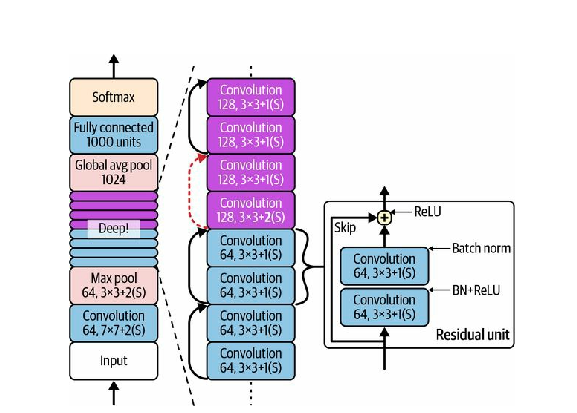
The idea of ResNet is simple to describe. It starts and ends exactly like GoogLeNet (except without a dropout layer), and in between is just a very deep stack of residual units. Each residual unit is composed of two (2) convolutional layers ^{23 23} There are no pooling layers , with batch normalization (BN) and ReLU activation, using 3-by-3 kernels and preserving spatial dimensions (stride of 1, "same" padding).

There are different variations of this aforementioned architecture, each having different numbers of layers. ResNet-34, as the name implies, is a ResNet with 34 layers (only counting the convolutional layers and the fully connected layer) containing 3 RUs that output 64 feature maps, 4 RUs with 128 maps, 6 RUs with 256 maps, and 3 RUs with 512 maps.

ResNets deeper than that, such as ResNet-152, use slightly different residual units. Instead of two (2) 3-by-3 convolutional layers with 256 feature maps, they use three (3) convolutional layers:

1.

a 1-by-1 convolutional layer with just 64 feature maps (4x less), which acts as a bottleneck layer (as discussed already)

2.

a 3-by-3 layer with 64 feature maps

3.

another 1-by-1 convolutional layer with 256 feature maps (4 times 64) that restores the original depth

ResNet-152 contains 3 such RUs that output 256 maps, then 8 RUs with 512 maps, a whopping 36 RUs with 1,024 maps, and finally 3 RUs with 2,048 maps.

7.7 Implementing a ResNet-34 CNN using Keras

Most CNN architectures described so far can be implemented easily using Keras ^{24 24} although generally we would load a pre-trained network instead, as we will see later. . To illustrate the process, let’s implement a ResNet-34 from scratch with Keras.

First, we’ll create a ResidualUnit layer:

DefaultConv2D = partial(tf.keras.layers.Conv2D, kernel_size=3, strides=1, 
                 padding="same", kernel_initializer="he_normal", 
                 use_bias=False) 
 
class ResidualUnit(tf.keras.layers.Layer): 
   def __init__(self, filters, strides=1, activation="relu", **kwargs): 
      super().__init__(**kwargs) 
      self.activation = tf.keras.activations.get(activation) 
      self.main_layers = [ 
         DefaultConv2D(filters, strides=strides), 
         tf.keras.layers.BatchNormalization(), 
         self.activation, 
         DefaultConv2D(filters), 
         tf.keras.layers.BatchNormalization() 
      ] 
      self.skip_layers = [] 
      if strides > 1: 
         self.skip_layers = [ 
           DefaultConv2D(filters, kernel_size=1, strides=strides), 
           tf.keras.layers.BatchNormalization() 
         ] 
 
   def call(self, inputs): 
      Z = inputs 
      for layer in self.main_layers: 
         Z = layer(Z) 
      skip_Z = inputs 
      for layer in self.skip_layers: 
         skip_Z = layer(skip_Z) 
      return self.activation(Z + skip_Z) 

As we can see, this code matches Figure 14-19 pretty closely. In the constructor, we create all the layers we will need:

Then in the call() method, we make the inputs go through the main layers and the skip layers ( if any ), and we add both outputs and apply the activation function.

Now we can build a ResNet-34 using a Sequential model , as it’s really just a long sequence of layers. We can treat each residual unit as a single layer now that we have the ResidualUnit class.

The code closely matches:

model = tf.keras.Sequential([ 
   DefaultConv2D(64, kernel_size=7, strides=2, input_shape=[224, 224, 3]), 
   tf.keras.layers.BatchNormalization(), 
   tf.keras.layers.Activation("relu"), 
   tf.keras.layers.MaxPool2D(pool_size=3, strides=2, padding="same"), 
]) 
prev_filters = 64 
for filters in [64] * 3 + [128] * 4 + [256] * 6 + [512] * 3: 
   strides = 1 if filters == prev_filters else 2 
   model.add(ResidualUnit(filters, strides=strides)) 
   prev_filters = filters 
 
model.add(tf.keras.layers.GlobalAvgPool2D()) 
model.add(tf.keras.layers.Flatten()) 
model.add(tf.keras.layers.Dense(10, activation="softmax"))

The only tricky part in this code is the loop that adds the ResidualUnit layers to the model. As explained earlier:

• the first 3 RUs have 64 filters,

• the next 4 RUs have 128 filters.

and so on. At each iteration, we must set the stride to 1 when the number of filters is the same as in the previous RU, or else we set it to 2; then we add the ResidualUnit, and finally we update prev_filters.

With just 40 lines of code, we can build the model that won the ILSVRC 2015 challenge. This demonstrates both the elegance of the ResNet model and the expressiveness of the Keras API. Implementing the other CNN architectures is a bit longer, but not much harder.

However, Keras comes with several of these architectures built in, so why not use them instead?

7.8 Using Pre-Trained Models from Keras

In general, we don’t have to implement standard models like GoogLeNet or ResNet manually, as pre-trained networks are readily available using the tf.keras.applications package.

For example, we can load the ResNet-50 model, pre-trained on ImageNet, with the following line of code:

import tensorflow as tf 
 
model = tf.keras.applications.ResNet50(weights="imagenet")

This was surprisingly simple. This will create a ResNet-50 model and download weights already trained on the ImageNet dataset. To use it, we first need to ensure the images have the correct size. A ResNet-50 model expects an image with the dimensions of 224-by-224-pixel ^{26 26} other models may expect other sizes, such as 299-by-299. , so let’s use the Resizing layer, provided by Keras, to resize two (2) sample images (after cropping them to the target aspect ratio):

from sklearn.datasets import load_sample_images 
 
K = tf.keras.backend 
images = K.constant(load_sample_images()["images"]) 
images_resized = tf.keras.layers.Resizing(height=224, width=224, 
                              crop_to_aspect_ratio=True)(images)

The pre-trained models assumes the images are pre-processed in a specific way. In some cases the models can expect the inputs to be scaled from 0 to 1, or from -1 to 1, and so on. Each model provides a preprocess_input() function we can use to pre-process our images. These functions assume the original pixel values range from 0 to 255, which is the case here:

inputs = tf.keras.applications.resnet50.preprocess_input(images_resized)

Now we can use the pre-trained model to make predictions:

Y_proba = model.predict(inputs) 
print(Y_proba.shape)

(2, 1000)

top_K = tf.keras.applications.resnet50.decode_predictions(Y_proba, top=3) 
for image_index in range(len(images)): 
   print(f"Image #{image_index}") 
   for class_id, name, y_proba in top_K[image_index]: 
      print(f"  {class_id} - {name:12s} {y_proba:.2%}")

The output looks like this:

Downloading data from https://storage.googleapis.com/download.tensorflow.org/data/imagenet_class_index.json 
Image #0 
  n03877845 - palace       54.69% 
  n03781244 - monastery    24.71% 
  n02825657 - bell_cote    18.55% 
Image #1 
  n04522168 - vase         32.67% 
  n11939491 - daisy        17.82% 
  n03530642 - honeycomb    12.04%

The correct classes are palace and dahlia (which you can see in Fig. 7.18 ), so the model is correct for the first image but wrong for the second .

Many vision models are available in tf.keras.applications, from lightweight and fast models to large and accurate ones. But what if we want to use an image classifier for classes of images that are not part of ImageNet? In that case, we may still benefit from the pre-trained models by using them to perform transfer learning .

7.9 Pre-Trained Models for Transfer Learning

If we want to build an image classifier but not have enough data to train it from scratch, it is often a good idea to reuse the lower layers of a pre-trained model [75]. For example, let’s train a model to classify pictures of flowers , reusing a pre-trained Xception model.

First, we’ll load the flowers dataset using TensorFlow Datasets:

import tensorflow_datasets as tfds 
 
dataset, info = tfds.load("tf_flowers", as_supervised=True, with_info=True) 
dataset_size = info.splits["train"].num_examples 
class_names = info.features["label"].names 
n_classes = info.features["label"].num_classes 
print(info)

test_set_raw, valid_set_raw, train_set_raw = tfds.load( 
   "tf_flowers", 
   split=["train[:10%]", "train[10%:25%]", "train[25%:]"], 
   as_supervised=True)

All three (3) datasets contain individual images. First let’s have a look at the data to get some idea on what we are working with.

We need to batch them, but first we need to ensure they all have the same size, otherwise batching will fail. We can use a Resizing layer for this. We must also call the tf.keras.applications. xception.preprocess_input() function to preprocess the images appropriately for the Xception model. Lastly, we’ll also shuffle the training set and use prefetching:

batch_size = 32 
preprocess = tf.keras.Sequential([ 
   tf.keras.layers.Resizing(height=224, width=224, crop_to_aspect_ratio=True), 
   tf.keras.layers.Lambda(tf.keras.applications.xception.preprocess_input) 
]) 
train_set = train_set_raw.map(lambda X, y: (preprocess(X), y)) 
train_set = train_set.shuffle(1000, seed=42).batch(batch_size).prefetch(1) 
valid_set = valid_set_raw.map(lambda X, y: (preprocess(X), y)).batch(batch_size) 
test_set = test_set_raw.map(lambda X, y: (preprocess(X), y)).batch(batch_size)

Now each batch contains 32 images, all of them 224-by-224 pixels, with pixel values ranging from -1 to 1.

This is the ideal values for training such a network. As the dataset is not very large, a bit of data augmentation will certainly help. Let’s create a data augmentation model that we will embed in our final model. During training, it will randomly flip the images horizontally, rotate them a little bit, and tweak the contrast:

data_augmentation = tf.keras.Sequential([ 
   tf.keras.layers.RandomFlip(mode="horizontal", seed=42), 
   tf.keras.layers.RandomRotation(factor=0.05, seed=42), 
   tf.keras.layers.RandomContrast(factor=0.2, seed=42) 
])

Next let’s load an Xception model, which is pre-trained on ImageNet. We exclude the top of the network by setting include_top=False. This excludes the global average pooling layer and the dense output layer. We then add our own global average pooling layer (feeding it the output of the base model), followed by a dense output layer with one unit per class, using the softmax activation function. Finally, we wrap all this in a Keras Model:

tf.random.set_seed(42)  # extra code  ensures reproducibility 
base_model = tf.keras.applications.xception.Xception(weights="imagenet", 
                                      include_top=False) 
avg = tf.keras.layers.GlobalAveragePooling2D()(base_model.output) 
output = tf.keras.layers.Dense(n_classes, activation="softmax")(avg) 
model = tf.keras.Model(inputs=base_model.input, outputs=output)

It’s usually a good idea to freeze the weights of the pre-trained layers, at least at the beginning of training ^{29 29} By not updating the weights of the frozen layers, we avoid tweaking features that are already well-established and generalize well across different tasks. :

for layer in base_model.layers: 
   layer.trainable = False

Finally, we can compile the model and start training:

optimizer = tf.keras.optimizers.SGD(learning_rate=0.1, momentum=0.9) 
model.compile(loss="sparse_categorical_crossentropy", optimizer=optimizer, 
          metrics=["accuracy"]) 
history = model.fit(train_set, validation_data=valid_set, epochs=3)

After training the model for a few epochs, its validation accuracy should reach a bit over 80% and then stop improving. This means that the top layers are now pretty well trained, and we are ready to unfreeze some of the base model’s top layers, then continue training.

For example, let’s unfreeze layers 56 and above (that’s the start of residual unit 7 out of 14, as you can see if you list the layer names):

for layer in base_model.layers[56:]: 
   layer.trainable = True

Don’t forget to compile the model whenever you freeze or unfreeze layers. Also make sure to use a much lower learning rate to avoid damaging the pre-trained weights:

optimizer = tf.keras.optimizers.SGD(learning_rate=0.01, momentum=0.9) 
model.compile(loss="sparse_categorical_crossentropy", optimizer=optimizer, 
          metrics=["accuracy"]) 
history = model.fit(train_set, validation_data=valid_set, epochs=10)

This model should reach around 92% accuracy on the test set, in just a few minutes of training (with a GPU). If you tune the hyperparameters, lower the learning rate, and train for quite a bit longer, you should be able to reach 95% to 97%.

But there’s more to computer vision than just classification. For example, what if you also want to know where the flower is in a picture? Let’s look at this now.

tf.random.set_seed(42)  # extra code  ensures reproducibility 
base_model = tf.keras.applications.xception.Xception(weights="imagenet", 
                                      include_top=False) 
avg = tf.keras.layers.GlobalAveragePooling2D()(base_model.output) 
class_output = tf.keras.layers.Dense(n_classes, activation="softmax")(avg) 
loc_output = tf.keras.layers.Dense(4)(avg) 
model = tf.keras.Model(inputs=base_model.input, 
                outputs=[class_output, loc_output]) 
optimizer = tf.keras.optimizers.SGD(learning_rate=0.01, momentum=0.9)  # added this line 
model.compile(loss=["sparse_categorical_crossentropy", "mse"], 
          loss_weights=[0.8, 0.2],  # depends on what you care most about 
          optimizer=optimizer, metrics=["accuracy", "mse"])