2

Decision Trees

2.1 Introduction

Decision Tree (DT) is a versatile ML algorithm which can perform both classification and regression tasks, and even multi-output tasks, capable of fitting complex datasets. They are classified as a non-parametric supervised learning algorithm, which is utilised for both classification and regression tasks.

It has a hierarchical tree structure, consisting of a root node, branches, internal nodes and leaf nodes. DT s are also the fundamental components of random forests, which are among the most powerful ML algorithms available today. Some of the applications include:

Loan Approval in Banking

Banks use DT s to assess whether a loan application should be approved. The decision is based on factors such as credit score, income, and loan history. This helps predict approval or rejection and enables quick and reliable decisions [1], [2].

Medical Diagnosis

In healthcare they assist in diagnosing diseases. For example, they can predict whether a patient has diabetes based on clinical data like glucose levels, Body-Mass Index (BMI) and blood pressure [3]. This helps classify patients into diabetic or non-diabetic categories, supporting early diagnosis and treatment [4].

Predicting Exam Results in Education

Educational institutions use to predict whether a student will pass or fail based on factors like attendance, study time and past grades. This helps teachers identify at-risk students and offer targeted support [5], [6].

Customer Churn Prediction

Companies use DT s to predict whether a customer will leave or stay based on behaviour patterns, purchase history, and interactions. This allows businesses to take proactive steps to retain customers [7].

Fraud Detection

In finance, DT s are used to detect fraudulent activities, such as credit card fraud [8]. By analysing past transaction data and patterns, DT s can identify suspicious activities and flag them for further investigation [9].

In this chapter we will start by discussing how to train, visualise, and make predictions with DT s. Then we will go through the Classification and Regression Tree (CART) training algorithm used by scikit-learn, and we will explore how to regularise trees and use them for regression tasks.

2.1.1 Advantages and Disadvantages

Before we start with our chapter on DT , lets list down the advantages it has over other methods:

Easy to Understand

DT s are visual which makes it easy to follow the decision-making process

Versatility

Can be used for both classification and regression problems.

No Need for Feature Scaling

Unlike many ML models, it doesn’t require us to scale or normalise our data.

Handles Non-linear Relationships

It capture complex, non-linear relationships between features and outcomes effectively.

Interpretability

The tree structure is easy to interpret helps in allowing users to understand the reasoning behind each decision.

Handles Missing Data

It can handle missing values by using strategies like assigning the most common value or ignoring missing data during splits.

Of course, as with every method, there are it’s disadvantages which are:

Over-fitting

They can over-fit the training data if they are too deep which means they memorise the data instead of learning general patterns. This leads to poor performance on unseen data.

Instability

It can be unstable which means that small changes in the data may lead to significant differences in the tree structure and predictions.

Bias towards Features with Many Categories

It can become biased toward features with many distinct values which focuses too much on them and potentially missing other important features which can reduce prediction accuracy.

Difficulty in Capturing Complex Interactions

DT s may struggle to capture complex interactions between features which helps in making them less effective for certain types of data.

Computationally Expensive for Large Datasets

For large datasets, building and pruning a DT can be computationally intensive, especially as the tree depth increases.

2.2 Training and Visualising Decision Trees

To understand DT s, let’s build one and take a look at how it makes predictions. The following code trains a DecisionTreeClassifier on the iris dataset:

from sklearn.datasets import load_iris 
from sklearn.tree import DecisionTreeClassifier 
iris = load_iris(as_frame=True) 
X_iris = iris.data[["petal length (cm)", "petal width (cm)"]].values 
y_iris = iris.target 
tree_clf = DecisionTreeClassifier(max_depth=2, random_state=42) 
tree_clf.fit(X_iris, y_iris)

We can visualise the trained DT by first using the export_graphviz() function to output a graph definition file called iris_tree.dot :

from sklearn.tree import export_graphviz 
export_graphviz( 
tree_clf, 
out_file="iris_tree.dot", 
feature_names=["petal length (cm)", "petal width (cm)"], 
class_names=iris.target_names, 
rounded=True, 
filled=True 
)

from graphviz import Source 
Source.from_file("iris_tree.dot")

2.3 Making Predictions

Let’s see how the tree represented in Fig. 2.1 makes predictions.

Suppose we find an iris flower and want to classify it based on its petals . Looking at our three in Fig. 2.1 , we start at the root node , which is depth 0, at the top. This node asks whether the flower’s petal length is smaller than 2,45 cm. If it is, then we move down to the root’s left child node , which is in this case it is depth 1, left, which is a leaf node , as in it does not have any child nodes, so it does not ask any questions as it simply look at the predicted class for that node, and the DT predicts that our flower is an Iris setosa (class=setosa).

Now suppose we find another flower, and this time the petal length is greater than 2,45 cm . We again start at the root but now move down to its right child node ^{1 1} which is depth 1, right . This is NOT a leaf node, it’s a split node , so it asks another question:

If it is, then our flower is most likely an Iris versicolor . If not, it is likely an Iris virginica .

A node’s samples attribute counts how many training instances it applies to.

A node’s value attribute tells us how many training instances of each class this node applies to.

For example, the bottom-right node applies to 0 Iris setosa, 1 Iris versicolor, and 45 Iris virginica.

Finally, a node’s gini attribute measures its Gini impurity , named after Corrado Gini ^{2 2} Corrado Gini ( 1884 - 1965 ) An Italian statistician, demographer and sociologist who developed the Gini coefficient, a measure of the income inequality in a society. Gini was a proponent of organicism and applied it to nations. which we will have a look at now.

2.3.1 Gini Impurity

Gini Impurity is a measurement used to build DT s to determine how the features of a dataset should split nodes to form the tree. More precisely, the Gini Impurity of a dataset is a number between 0 - 0.5, which indicates the likelihood of new, random data being misclassified if it were given a random class label according to the class distribution in the dataset.

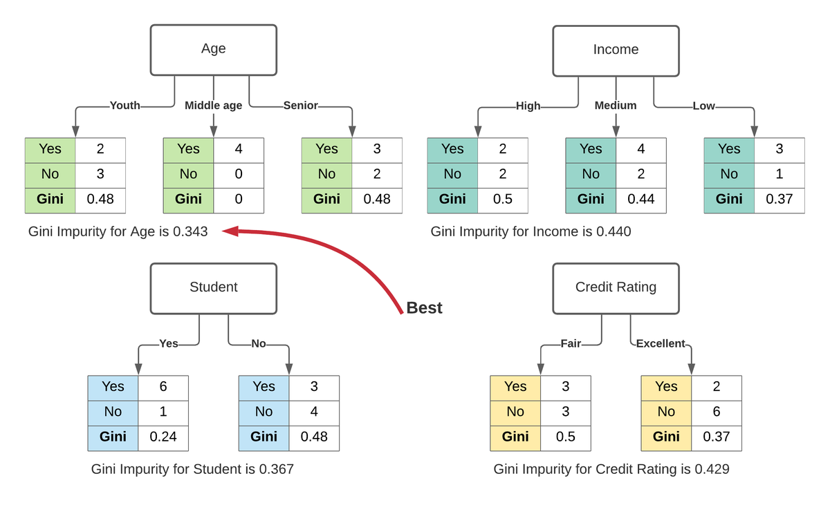
For example, say we want to build a classifier which determines if someone will default on their credit card. We have some labelled data with features, such as bins for age, income, credit rating, and whether or not each person is a student. For us to find the best feature for the first split of the tree ^{3 3} i.e., the root node we could calculate how poorly each feature divided the data into the correct class:

• default ("yes"), or

• didn’t default ("no").

This calculation would measure the impurity of the split, and the feature with the lowest impurity would determine the best feature for splitting the current node. This process would continue for each subsequent node using the remaining features.

In Fig. 2.2 , age has minimum Gini impurity, so age is selected as the root in the decision tree.

Going back to our iris flower example, since the depth-1 left node applies only to Iris setosa training instances, it is pure and its Gini impurity is 0. Eq. ( 2.1 ) shows how the training algorithm computes the Gini impurity $G_i^{}$ of the $i_{}^{th}$ node. The depth-2 left node has a Gini impurity of

Mathematically we can define the Gini impurity as:

where $G_i^{}$ is the Gini impurity of the $i_{}^{th}$ node, $p_{i,k}^{}$ is the ratio of class $k$ instances among the training instances in the $i_{}^{th}$ node. Using this definition we can calculate the depth-2 left node as:

scikit-learn uses the CART algorithm, which produces only binary trees , meaning trees where split nodes always have exactly two (2) children. ^{4 4} i.e., questions only have yes/no answers.

Fig. 2.3 shows this DT ’s decision boundaries. The thick vertical line represents the decision boundary of the root node (depth 0) with petal length = 2,45cm. Given the left hand area is pure (only Iris setosa ), it cannot be split any further. However, the right hand area is impure , so the depth-1 right node splits it at petal width = 1,75cm, which is represented by the dashed line.

Given max_depth was set to 2, the DT stops right there. If we set max_depth to 3, then the two depth-2 nodes would each add another decision boundary. ^{6 6} Which is represented by the two vertical dotted lines.

2.3.2 Estimating Class Probabilities

A DT can also estimate the probability which an instance belongs to a particular class $k$ . First, it traverses the tree to find the leaf node for this instance, and then it returns the ratio of training instances of class $k$ in this node.

For example, suppose we have found a flower whose petals are 5cm long and 1,5cm wide. The corresponding leaf node is the depth-2 left node, so the DT outputs the following probabilities:

• 0% for Iris setosa (0/54),

• 90.7% for Iris versicolor (49/54), and

• 9.3% for Iris virginica (5/54).

If we ask it to predict the class, it outputs Iris versicolor (class 1) because it has the highest probability . Let’s check this:

print(tree_clf.predict_proba([[5, 1.5]]).round(3)) 
print(tree_clf.predict([[5, 1.5]]))

[[0.    0.907 0.093]] 
[1]

Notice the estimated probabilities would be identical anywhere else in the bottom-right rectangle of Fig. 2.1 , for example, if the petals were 6cm long and 1,5cm wide.

2.4 The CART Training Algorithm

CART is a predictive algorithm used for explaining how the target variable’s values can be predicted based on other matters. It is a DT where each fork is split into a predictor variable and each node has a prediction for the target variable at the end. The three (3) primary points of the algorithm is as follows:

Tree structure

CART builds a tree-like structure consisting of nodes and branches. The nodes represent different decision points, and the branches represent the possible outcomes of those decisions. The leaf nodes in the tree contain a predicted class label or value for the target variable.

Splitting Criteria

CART uses a greedy approach to split the data at each node. It evaluates all possible splits and selects the one that best reduces the impurity of the resulting subsets. For classification tasks, CART uses Gini impurity as the splitting criterion. The lower the Gini impurity, the more pure the subset is. For regression tasks, CART uses residual reduction as the splitting criterion. The lower the residual reduction, the better the fit of the model to the data.

Pruning

To prevent over-fitting of the data, pruning is a technique used to remove the nodes that contribute little to the model accuracy. Cost complexity pruning and information gain pruning are two popular pruning techniques. Cost complexity pruning involves calculating the cost of each node and removing nodes that have a negative cost. Information gain pruning involves calculating the information gain of each node and removing nodes that have a low information gain.

scikit-learn uses the CART algorithm to train DT s (also called growing trees). The algorithm works by splitting the training set into two (2) subsets using a single feature $k$ and a threshold $t_k^{}$ . ^{7 7} e.g., petal length $\le$ 2,45 cm .

How does it choose $k$ and $t_k^{}$ ?

It searches for the pair ${\left(k,t_k^{}\right)}^{}$ that produces the purest subsets, weighted by their size. Eq. ( 2.2 ) gives the cost function that the algorithm tries to minimise.

Once the CART algorithm successfully splits the training set in two, it splits the subsets using the same logic, then the sub-subsets, and so on, recursively. It stops its recursive behaviour once it reaches the maximum depth, ^{8 8} defined by the max_depth hyperparameter. or if it cannot find a split that will reduce impurity.

A few other hyperparameters control additional stopping conditions:

2.4.1 Gini Impurity v. Information Entropy

By default, the DecisionTreeClassifier class uses the Gini impurity measure, but we can select the entropy impurity measure instead by setting the criterion hyperparameter to entropy .

In ML , entropy is frequently used as a measurement of impurity, a set’s entropy is zero when it contains instances of only one class. Eq. ( 2.3 ) shows the definition of the entropy of the $i_{}^{th}$ node.

For example, the depth-2 left node in Fig. 2.1 has an entropy equal to:

And the general equation for entropy could be written as:

Most of the time it does not make a big difference as they lead to similar trees. Gini impurity is slightly faster to compute, so it is a good default. However, when they differ, Gini impurity tends to isolate the most frequent class in its own branch of the tree, while entropy tends to produce slightly more balanced trees.

2.4.2 Regularisation Hyperparameters

DT s make very few assumptions about the training data. ^{10 10} as opposed to linear models, which assume that the data is linear, for example If left unconstrained, the tree structure will adapt itself to the training data, fitting it very closely-indeed, resulting in over-fitting .

Such a model is often called a non-parametric model, not because it does not have any parameters ^{11 11} as it often has a lot. but because the number of parameters is not determined prior to training, so the model structure is free to stick closely to the data.

In contrast, a parametric model, such as a linear model, has a predetermined number of parameters, so its degree of freedom is limited, reducing the risk of over-fitting.

To avoid over-fitting the training data, we need to restrict the DT ’s freedom during training. As we should know by now, this is called regularisation .

The regularisation hyperparameters depend on the algorithm used, but generally we can at least restrict the maximum depth of the DT . In scikit-learn, this is controlled by the max_depth hyperparameter. The default value is None, which means unlimited. Reducing max_depth will regularise the model and thus reduce the risk of over-fitting.

The DecisionTreeClassifier class has a few other parameters that similarly restrict the shape of the DT :

max_features

Maximum number of features that are evaluated for splitting at each node

max_leaf_nodes

Maximum number of leaf nodes

min_samples_split

Minimum number of samples a node must have before it can be split

min_samples_leaf

Minimum number of samples a leaf node must have to be created

min_weight_fraction_leaf

Same as min_samples_leaf but expressed as a fraction of the total number of weighted instances.

Let’s test regularisation on the moons dataset, introduced previously. We’ll train one DT without regularisation, and another with min_samples_leaf=5. Here’s the code with Fig. 2.4 showing the decision boundaries of each tree.

from sklearn.datasets import make_moons 
 
X_moons, y_moons = make_moons(n_samples=150, noise=0.2, random_state=42) 
 
tree_clf1 = DecisionTreeClassifier(random_state=42) 
tree_clf2 = DecisionTreeClassifier(min_samples_leaf=5, random_state=42) 
tree_clf1.fit(X_moons, y_moons) 
tree_clf2.fit(X_moons, y_moons)

The unregulated model on the left is clearly over-fitting, and the regularised model on the right will probably generalise better. We can verify this by evaluating both trees on a test set generated using a different random seed:

X_moons_test, y_moons_test = make_moons(n_samples=1000, noise=0.2, random_state=43) 
print(tree_clf1.score(X_moons_test, y_moons_test)) 
print(tree_clf2.score(X_moons_test, y_moons_test))

0.898 
0.92

As we can see, the ${\text{2}}^{\text{nd}}$ tree has a better accuracy on the test set.

2.5 Regression

DT s are also capable of performing regression tasks. Let’s build a regression tree with the DecisionTreeRegressor class, training it on a noisy quadratic dataset with max_depth=2 with the resulting tree being represented in Fig. 2.5 .

This tree looks very similar to the classification tree built earlier. The main difference is that instead of predicting a class in each node, it predicts a value .

For example, say we want to make a prediction for a new instance with $x_1^{}$ = 0.2. The root node asks whether $x_1^{}\le 0.197$ . As it is not, the algorithm goes to the right child node, which asks whether $x_1^{}\le 0.772$ . Since it is, the algorithm goes to the left child node. This is a leaf node, and it predicts value=0.111. This prediction is the average target value of the 110 training instances associated with this leaf node, and results in a mean squared error equal to 0.015 over these 110 instances.

This model’s predictions are represented on the left in Fig. 2.6 . If we set max_depth=3, we get the predictions represented on the right. Notice how the predicted value for each region is always the average target value of the instances in that region. The algorithm splits each region in a way that makes most training instances as close as possible to that predicted value.

The CART algorithm works as described earlier, except that instead of trying to split the training set in a way that minimises impurity, it now tries to split the training set in a way that minimises the Mean Square Error (MSE) . To get a better feel of the underlying mathematics, Eq. ( 2.4 ) shows the cost function that the algorithm tries to minimise:

Just like for classification tasks, DT s are prone to over-fitting when dealing with regression tasks. Without any regularization, ^{12 12} i.e., using the default hyperparameters. we get the predictions on the left in Fig. 2.7 .

As can clearly be seen, these predictions are over-fitting the training set very badly. Setting min_samples_leaf=10 results in a significantly more reasonable model, represented on the right in Fig. 2.7 .

2.6 Sensitivity to Axis Orientation

DT s have a lot going for them given they are relatively easy to understand and interpret, simple to use, versatile, and powerful. However, they do have a few limitations. First, as we may have noticed, DT s love orthogonal decision boundaries, ^{13 13} all splits are perpendicular to an axis. which makes them sensitive to the orientation of data.

For example, Fig. 2.8 shows a simple linearly separable dataset where on the left, a DT can split it easily, while on the right, after the dataset is rotated by 45 degrees, the decision boundary looks unnecessarily convoluted. Although both DT s fit the training set perfectly, it is very likely that the model on the right will not generalise well.

One way to limit this problem is to scale the data, then apply a principal component analysis transformation. We will look at Principal Component Analysis (PCA) in detail later, but for now we only need to know that it rotates the data in a way that reduces the correlation between the features, which often makes things easier for trees.

Let’s create a small pipeline that scales the data and rotates it using PCA , then, continue on to train a DecisionTreeClassifier on that data.

from sklearn.decomposition import PCA 
from sklearn.pipeline import make_pipeline 
from sklearn.preprocessing import StandardScaler 
 
pca_pipeline = make_pipeline(StandardScaler(), PCA()) 
X_iris_rotated = pca_pipeline.fit_transform(X_iris) 
tree_clf_pca = DecisionTreeClassifier(max_depth=2, random_state=42) 
tree_clf_pca.fit(X_iris_rotated, y_iris)

Fig. 2.9 shows the decision boundaries of that tree and as we can see, the rotation makes it possible to fit the dataset pretty well using only one (1) feature, which is a linear function of the original petal length and width.